

1. Introduction
2. DIC technology
2.1 Background
2.2 Principle of 2D-DIC
2.3 Application of DIC technique
3. Application of DIC on Geotechnical Tests
3.1 Footing test
3.2 Trapdoor test
3.3 Retaining wall test
3.4 Wide width test on geogrid
3.5 DIC Procedure (Data acquisition and analysis)
4. Results and Discussion
4.1 Validation of DIC results
4.2 Soil displacement and strains
4.3 Geogrid strains
5. Conclusions
1. Introduction
The local deformation of soil, such as the formation mechanism of shear zone and progressive failure characteristics, is an important property of soil different from conventional continuous media (Luque and Bray, 2017). It can lead to socially and economically catastrophic events due to localized shear failure of the soil (Petley, 2012). Therefore, the study of soil tests has important theoretical significance and practical value for improving the theory of computational soil mechanics and preventing foundation engineering disasters. In order to have a comprehensive and detailed understanding of the local deformation and failure law of the soil, a large number of scholars have carried out a lot of research work from the aspects of theoretical methods (Terzaghi et al., 1996), numerical simulation (Han and Gabr, 2002; Lai et al., 2020; Liao and Yang, 2021; Tan et al., 2020), and experimental methods (Burke and Elshafie, 2021; Michalowski and Shi, 2003).
The laboratory test is an important means to obtain the deformation and failure characteristics of soil structure. For the measurement of soil deformation, multiple technologies are used to obtain the deformation and local strain behavior. In the traditional method, displacement transducers are used to measure the surface displacement (Liu et al., 2017; Yao and Takemura, 2019), and CT scanning is used to obtain the local strain and volume strain (Alikarami et al., 2014; Cheng and Wang, 2019).
Digital image correlation (DIC) was first proposed in the 1980s (Peters et al., 1983). With the development of computer technology, its theoretical algorithm and accuracy have been greatly improved. Compared with sensor contact measurement and external radiation measurement, digital image correlation has many advantages: the measurement system has low requirements for the environment, and only speckle and light source needs to be arranged on the sample surface; the acquisition process is non-contact measurement and highly automated, which will not affect the test. The whole field displacement and strain can be obtained with high measurement accuracy; The test process can be reproduced by animation. Therefore, digital image correlation has been applied to the field of geotechnical engineering. Zhao et al. (2021) obtained the soil displacement field by using the self-made trapdoor device and Particle Image Velocimetry (PIV) system and introduced the evolution law of deep and shallow buried displacement respectively. Khatami et al. (2019) used DIC to study the active arching effect in soil and obtained the distribution of vertical strain and horizontal strain and the change of earth pressure.
In this study, the application of advanced digital image correlation (DIC) technology in the geotechnical tests, such as shallow footing bearing capacity test, trapdoor test, retaining wall test, and wide width tensile test is demonstrated. Relevant reduced-scale model tests were performed using standard sand while applying the DIC technique to capture the soil movement during tests. A commercially available proprietary DIC software, VIC-2D, was used for digital correlation of captured images during the tests to generate soil displacements and strains. The results show that the DIC technique can capture the ground deformation field and associated failure patterns reasonably well when compared with the theoretical ones. Additional tests on geogrid also confirmed that the DIC technique is also appropriate to be used for the wide width tensile test on geogrid, It is demonstrated in this study that the advanced DIC technique can be effectively used in monitoring the deformation and strain field during a reduced-scale geotechnical model laboratory test.
2. DIC technology
2.1 Background
Digital image correlation method is a real-time, dynamic, and non-contact full field deformation optical measurement method, also known as digital image speckle correlation method. Since it was invented in the 1980s, many scholars have conducted in-depth research on it, and constantly innovated and improved the algorithm and application, so that the digital image correlation method maintains a sustained and rapid development and is widely used in many fields, mainly for the full field measurement of morphology, deformation, and strain (Blaber et al., 2015; Gao et al., 2015). At present, many companies and researchers have developed DIC algorithms for evaluating displacement and strain. For example, VIC-2D system and VIC-3D system were developed by Correlated Solutions Company, Q-400 system developed by Dante Dynamics Company, the Matlab-based open-source DIC software Ncorr developed by Blaber et al. (2015), and the free software Geo -PIV developed by Stanier (Blaber et al., 2015; Khatami et al., 2019; Stanier et al., 2016). Whether the DIC method measures in-plane deformation and displacement or three-dimensional deformation and displacement, it can be classified as 2D-DIC method and 3D-DIC. The experimental research content of this paper represents the plane strain problem, so the VIC-2D system from Correlated Solutions is adopted.
2.2 Principle of 2D-DIC
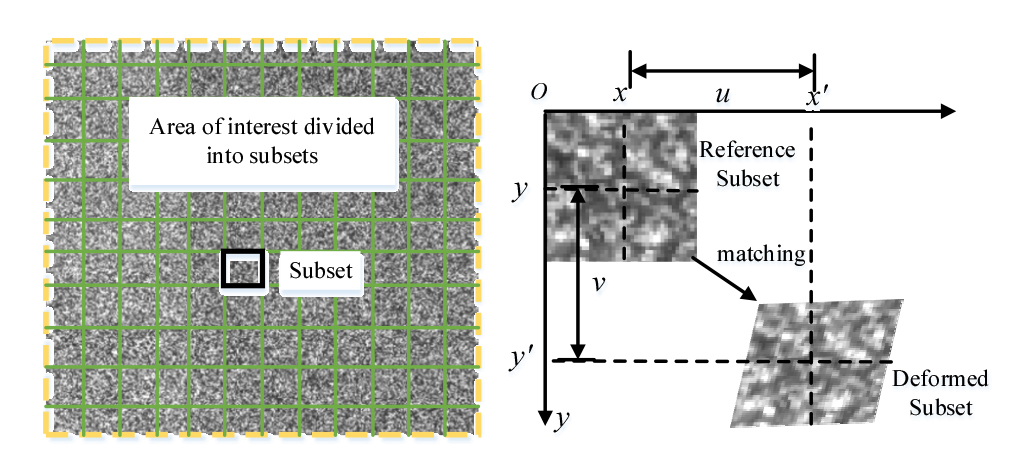
The basic principle of the digital image correlation measurement method is based on the image with certain distribution feature points, which is called a speckle image. Each pixel in speckle image corresponds to different light intensity, which is called gray value. These feature points take pixel points as coordinates and pixel gray as information carriers. The scattered speckle distributed on the surface of the object under test will move with the deformation of the object, and the deformation of the object under test can be obtained by tracking the change of grayscale, and this matching method is called grayscale matching. Before running the correlation algorithm, the area of interest (AOI) is selected as the computation area in the acquired reference image and divided into several computation window subsets, which are (2M + 1)×(2M + 1) pixel rectangles with the points (x, y) as the center of the point to be computed.
The functional relationship between a point (x, y) in the reference image and its corresponding point (x', y') in the deformed target image is as follows:
Where u and v are the displacements of the center of the reference image subset in the x and y directions; Δx and Δy are the distance from the point (x, y) to the center of the subset.
All pixels in the AOI before and after deformation are matched one by one, the appropriate correlation function is selected for correlation calculation, which is called the correlation formula (Pitas, 2000). Because the zero-mean normalized cross-correlation criterion (ZNCC) has the advantages of high matching accuracy and insensitivity to the effect of illumination, it is used as the evaluation function for the similarity between the reference image subset and the target image subset (Pan et al., 2009). The details of the theory related to ZNCC can be found elsewhere (Dematteis and Giordan, 2021)
The area where the correlation coefficient with the reference image window is the extreme value is found in the deformed image, and the found deformed image subset centered on (x', y') is the matching region of the deformed image corresponding to the reference image. Finally, the displacements u and v of the point to be calculated in the x and y directions can be obtained. As shown in Fig. 1. After analyzing the displacement vector of the center point of multiple subsets, the displacement field of the whole analysis region is formed.
The displacement search process of the measurement method is generally divided into two parts: whole pixel search and Sub-pixel Search. Due to the discreteness of digital images, it is easy to calculate the integer displacement with one pixel as the precision unit. To obtain the sub-pixel accuracy, the two-dimensional digital image correlation algorithm needs to complete two steps: setting the initial value and measuring the sub-pixel displacement. At present, the commonly used Sub-pixel Search algorithm is the method. For this method, the setting of the initial value is very important. It can converge only after the accurate initial value is determined. For the coarse and fine search method and peak search method, before the sub-pixel displacement search algorithm, it is necessary to provide an integer displacement of pixel resolution as the initial setting value of Sub-pixel Search.
2.3 Application of DIC technique
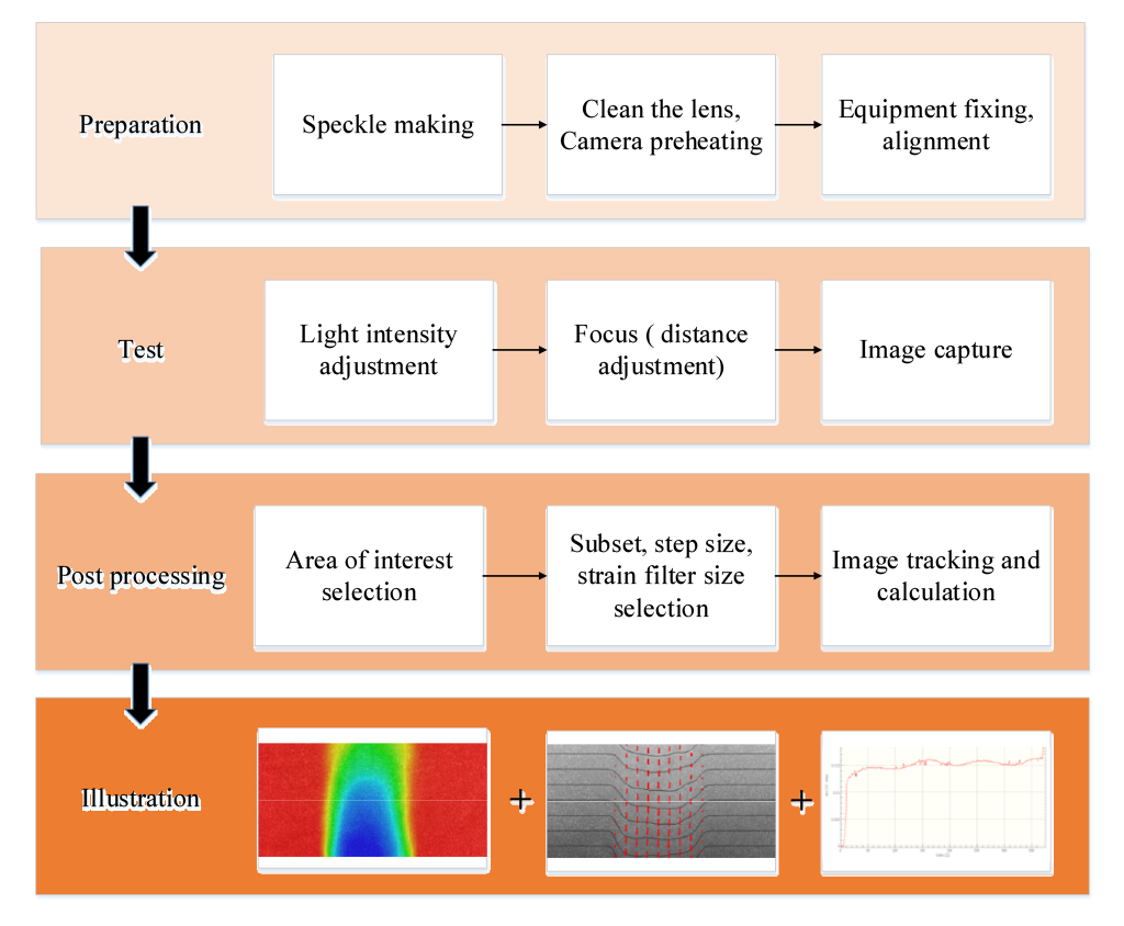
The experimental process of the digital image correlation method includes three parts: specimen preparation, image acquisition process, and image analysis.
As DIC method is to obtain deformation information by analyzing the grayscale features of digital images on the surface of the specimen, the surface of the specimen must have a random grayscale distribution that can carry deformation information and change accordingly with the deformation of the object, i.e., random speckle. There are two methods to obtain the scattered spots in the experiment; (1) artificially making speckles on the surface of the specimen by staining, painting, etc.; (2) the natural texture on the surface of the specimen. According to the specific requirements of the experiment and the specimen, we can choose the appropriate scattered speckles.
In this study, the 2D-DIC system developed by Correlated Solutions was used. The system consists of a hardware system responsible for taking pictures and a software system responsible for photo acquisition setup and processing analysis. The hardware system mainly includes a camera, lens, tripod, lighting, and standard device. The resolution of the camera is 2448×2048 pixels and the focal length is 8 mm. The main steps of the test are as follows: the CCD industrial camera is placed directly in front of the specimen scatter and the tripod height is adjusted to the same height as the specimen. LED lights are placed on both sides of the specimen to provide a stable light source; the software system includes VIC-Snap software and VIC-2D software. VIC-Snap is the software that controls the image acquisition, which can adjust the imaging speed and exposure time, allowing users to customize the image acquisition time and frequency.
After the test, the collected digital speckle image is imported into the DIC data analysis software VIC-2D. In the post-processing process, size calibration is usually the first step, and then the area of interest can be defined and the subset size. The undeformed speckle image before the test is used as a reference for calculating the surface deformation field of the sample. In order to obtain the global displacement and strain, the calculation area is usually set to cover the whole surface of the specimen. Fig. 2 shows a flow chart of the DIC application process.
3. Application of DIC on Geotechnical Tests
Four different types of tests were considered in this study, namely, 1) footing test; 2) trap-door test; 3) retaining wall test, and 4) wide-width tensile test on geogrid. Details of the test setups are given in this section
3.1 Footing test
3.1.1 Test setup
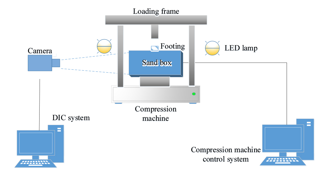
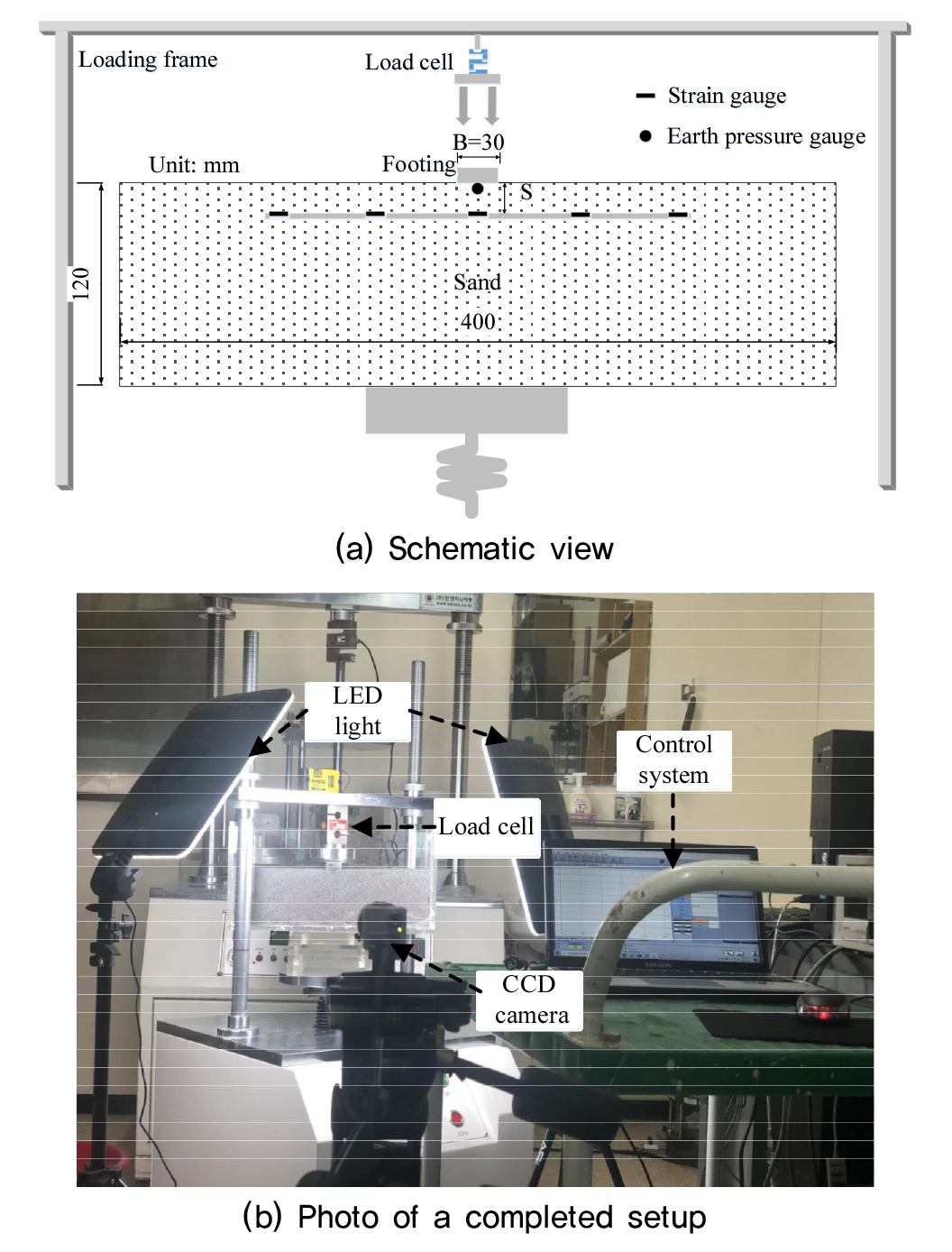
The footing test was performed in a plane strain condition. The test system consists of a sandbox, a loading system, a digital camera, two LED lamps, and two computers. The sandbox is a rigid cuboid container assembled from transparent plexiglass plates with an internal dimension of 400×150×200 mm (length×width×height). The soil movement and shear failure zone during loading through the plexiglass plate can be observed by a digital camera. The loading system includes a loading machine, computer control system, and footing. The loading platform moves upward at a speed of 6 mm/min and is controlled by the system during the test. The control system records the displacement of the footing at the same time. The width (B) of footing is 30mm and the length is 148mm. The length is slightly smaller than the internal width of the sandbox, with a gap of 1mm from both sides of the sandbox, which can effectively reduce the friction between the footing and plexiglass plate (Chen et al., 2021; Tafreshi and Dawson, 2010). Two LED lights were placed on both sides of the sandbox to provide the light source. A digital camera was at the same height as the sandbox to capture the test photos. Fig. 3 shows the schematic of the test device.
In the test, the test box was carefully filled in layers, 20 mm thick each, with a mixture of dyed and regular sand while being mildly compacted and leveled with a tamper to a target unit weight of 16.5 kN/m3. The sand particles were randomly poured into the sandbox, which facilitates the creation of a specimen with a minimal internal structure that would otherwise significantly affect test results. Repeat the above operation until the sand filling height reaches the design height. The compression machine records the changes of the footing load and displacement every 0.5s using an internally devised load cell and a LVDT. The digital camera also captures photos at the same frequency as the compression (Fig. 4).
3.1.2 Model ground and speckle preparation
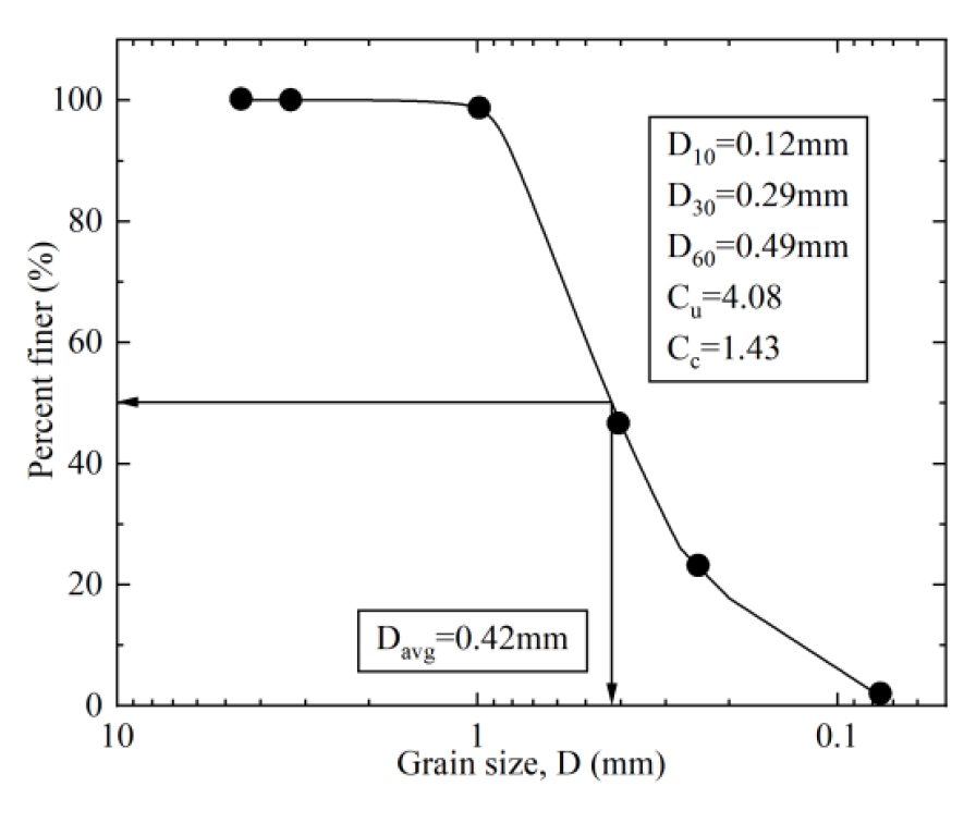
Fine-graded sand provided by Hi-Tech, South Korea was used to form the model sand bed having a relative density of 80%. The sand, classified as SP according to the Unified Soil Classification System (USCS), per ASTM D2487-17 (2017), has the effective size (D10), uniformity coefficient (Cu), and coefficient of curvature (Cc) of (0.12 mm, 4.08, and 1.43), respectively. The minimum and maximum dry unit weights are γd,min = 14.8 kN/m3, and γd,max = 17.0 kN/m3, respectively. Fig. 5 shows the grain size distribution curve.
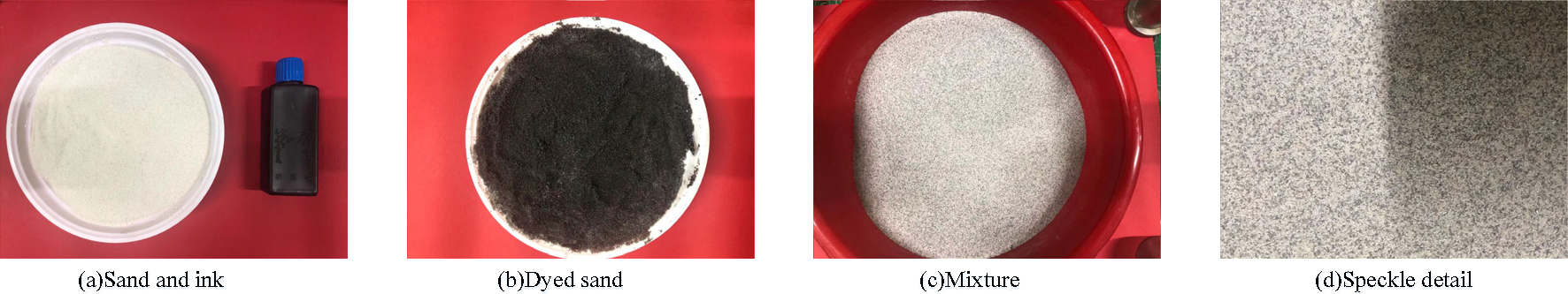
The sand particles used in the test were naturally yellowish in color, which are too bright and are considered not suitable for DIC analysis. Therefore, in order to increase traceability of soil particle movement by image analysis algorism in the DIC analysis, special care was needed in preparing the soil. As a first step of the experiment, the sand was dyed to obtain high contrast and random speckle. To achieve this goal, about half of the sand is dyed with matte black paint. It is left to stand for 48 hours and then mixed thoroughly with the remaining sand. The process of speckle is presented in Fig. 6.
3.2 Trapdoor test
3.2.1 Test setup
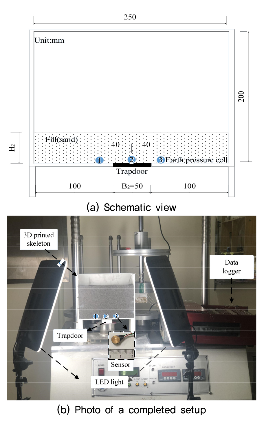
The trapdoor test box is composed of a 3D printed frame and a transparent plexiglass plate. The front wall of the test box is a transparent plexiglass plate to ensure optimal imaging of soil movement during the experiment, which is polished smooth enough to reduce the impact of friction on the test results. The internal dimensions of the test box are 250 mm in length, 65 mm in width, and 200 mm in height. The trapdoor was installed at the bottom and center of the test box with a dimension of a width of 50 mm and a length of 65 mm.
The change of pressure was monitored using the three earth pressure cells placed near the trap door at the location immediately above the trapdoor and at the stable parts on both sides, as shown in Fig. 7(a). The pressure sensors manufactured by Tokyo Measuring Instruments Lab were used, having a cylindrical shape with a radius of 3.8mm and a height of 2mm with a maximum measuring range of 100 kPa. Data were collected using a data logger at a sampling interval of 1s. The arrangement of the test setup is shown in Fig. 7(b). Similar steps used in the footing test were taken in preparing the soil.
3.2.2 Model preparation
The sand was filled in the test box in layers (20 mm thick each) by gently compacting to have a target unit weight of 15.5 kN/m3, which corresponds to the relative density of 35% representing a loose state. After start of the test with the DIC setup, photos were taken at intermittent steps after moving the trap door down for a certain distance. The test was completed when the trap door movement reached 30 mm. The initial height of the trap door (H2) was varied at H2/B2=2 and 3 where B is the width of the trap door. This corresponds to a shallow trapdoor test and a deep trapdoor test, respectively, Dewoolkar et al. (2007). Table 1 summarizes the scheme of the trapdoor tests.
Table 1.
Scheme of the trap door tests
| Test No. |
Width of trapdoor (B2/mm) |
Filling height (H2/mm) |
Embedment ratios (H2/B2) |
| 1 (shallow condition) | 50 | 100 | 2.0 |
| 2 (deep condition) | 150 | 3.0 |
3.3 Retaining wall test
3.3.1 Test setup
Retaining wall tests were carried out in a test box, made of a 20 mm thick plexiglass, having an internal dimension of 360 mm long, 250 mm high, and 140 mm wide. The same sand was used as backfill material in the test, which is the same as the previous test. The sand has a unit weight of 15.5 kN/m3 and a relative density of 35%, which corresponds to a loose state, and the internal friction angle Φ is taken to be 30% (Das, 2021). The wall (H3=150 mm) was also made with the same plexiglass of the same thickness was sufficiently rigid to yield active as well as passive states. Three earth pressure gauges were installed at 50, 75, and 100 mm from the top of the backfill soil to measure the horizontal earth pressure acting on the wall (Fig. 8).
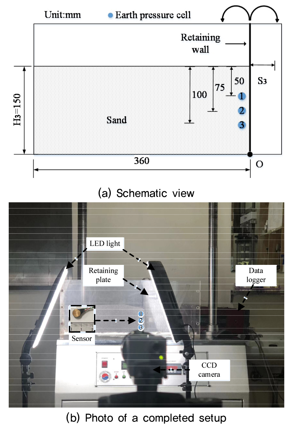
Both active and passive states were induced by moving the wall in opposite directions In the initial state, the retaining plate on the right side of the model is vertical. The retaining wall fact in contact with the soil was made plate smooth and allowed to rotate at the toe by hinge connection. To observe the active state formation of the backfill soil, the wall was rotated away from the backfill soil until the rotation angle reached 15 degrees with the soil movement being photographed every 1 degree of rotation. Similarly, the passive state was achieved by rotating the wall into the backfill soil to a maximum angle of 15 degrees at the top of the wall. As for the monitoring of earth pressure, previous studies have shown that these preset movements of retaining were sufficient to yield active and passive states (Fang et al., 1994; Mei et al., 2009; Ni et al., 2018).
3.4 Wide width test on geogrid
A wide width tensile test on a geogrid was also considered to investigate the applicability of the DIC technique as shown in Fig. 9. A polyethylene geogrid with 30 mm×30 mm aperture was used for testing, following ASTM D6637/D6637M-15 (2015). As shown in the test setup configuration, a geogrid specimen of 225 mm (width) ×300 mm (length) was loaded in tension using a hydraulic loading system capable of applying monotonic, sustained, and cyclic loading.
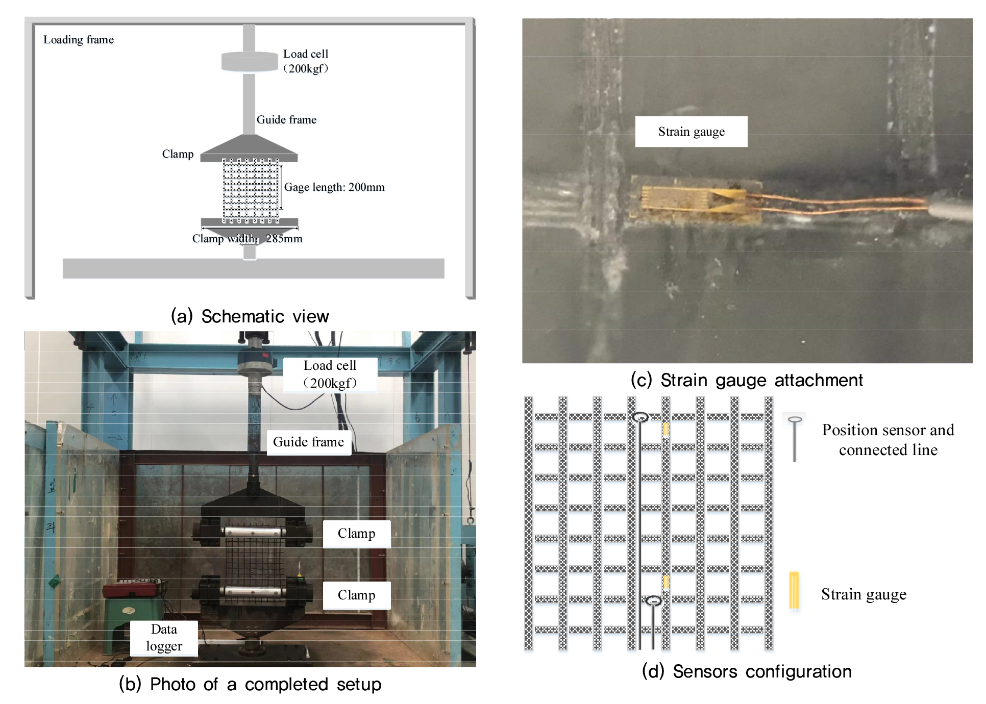
In this test, the 3-wire quarter-bridge strain gauges (SG) made by Tokyo Measuring Instruments Laboratory and the side-driven position sensors (PS) made by Novotechnik were installed to the polypropylene geogrid. Strain gauges are used to obtain local strain on the geogrid, while position sensors record changes in relative position to obtain global strain. Preparation of geogrid specimens that are suitable for application of the DIC technique was even more trickier than that for soil as target geogrid elements have limited area making it difficult to trace relevant movement. In the specimen preparation, an optimized procedure was developed in preparing test specimens in terms of applying speckles. To create a clear digital signal on the surface of the geogrid that can be recognized by the DIC system, white paint is sprayed on the surface to create a uniform base color. Then the black paint is sprayed at a distance of 50 cm from the specimen, horizontally to form a uniform speckle. Too bright or too dark paint will affect the quality of speckle, so only a small amount of work at a time and a light spray will help reduce this possibility.
3.5 DIC Procedure (Data acquisition and analysis)
As mentioned previously, the DIC analysis procedure includes setting up the reference image, calibration for scales, selection of parameters, and analysis. Detailed procedures are illustrated for the footing and the wide width tests.
3.5.1 Footing test, trapdoor test, and retaining wall test
A reference image should be selected first so that ground strains and displacements can be related to this image. By default, the reference image is on the first image in the sequence. However, for the tracking of sand particles, the incremental correlation function was used. This compares each image to a previous image rather than comparing each image to a reference image, which can lead to an increase in error, but in this experiment, this helps track the sliding of sand particles better. The area of interest is then selected in the next step, which contains a number of square patches of the same size. These square patches are called subsets. It is known that the size of the subset and the calculation step determine the accuracy and the cost of the calculation. In the VID-2D program, the program gives a recommended subset size based more on the quality of the speckle. Each subset should contain enough black and white pixel information to be distinguishable from other subsets. The step size is usually one-quarter of the subset size and using the default value gives satisfactory results. After the above parameters have been set, two points with known distances are manually selected for dimensional calibration, thus converting pixel information into distance information. According to the above steps, the subset size and the step size are selected as, 29×29 pixels and 7, respectively. In calculating strains, the Lagrangian strain tensor is used with a strain filter size of 15.
3.5.2 Wide width test
In a wide tensile test, the photo before tensile is selected as the reference image, and all images during tensile are compared with the first image to track the relevant motion. Due to the limited width of the rib, the default settings make it difficult to track the correlation motion. Using the fill boundary function helps get a lot more data closer to the edges.
Different from the soil test, a smaller subset needs to be selected for the tensile test on geogrid. Although a large subset contains enough grey-scale information, it also means a smaller number of subsets and a smaller degree of accuracy in the deformation results, which can lead to ribs that cannot be tracked. The smaller subsets produce a noisy deformation effect and therefore finer patches are produced (Pan et al., 2008). Accordingly, choose small step sizes so that the algorithm will work best.
For the calculation of strains in geogrid, the use of the Lagrangian strain tensor in the case of large strains overestimates the strain due to higher-order terms and therefore the engineering strain is chosen. The total smoothed area is the product of the step size and the strain filter size. Small step size was chosen in the previous step, requiring a rather larger strain filter size of 75. According to the above steps, the subset size was selected as 9×9 pixels while the step size of 1 was used.
4. Results and Discussion
4.1 Validation of DIC results
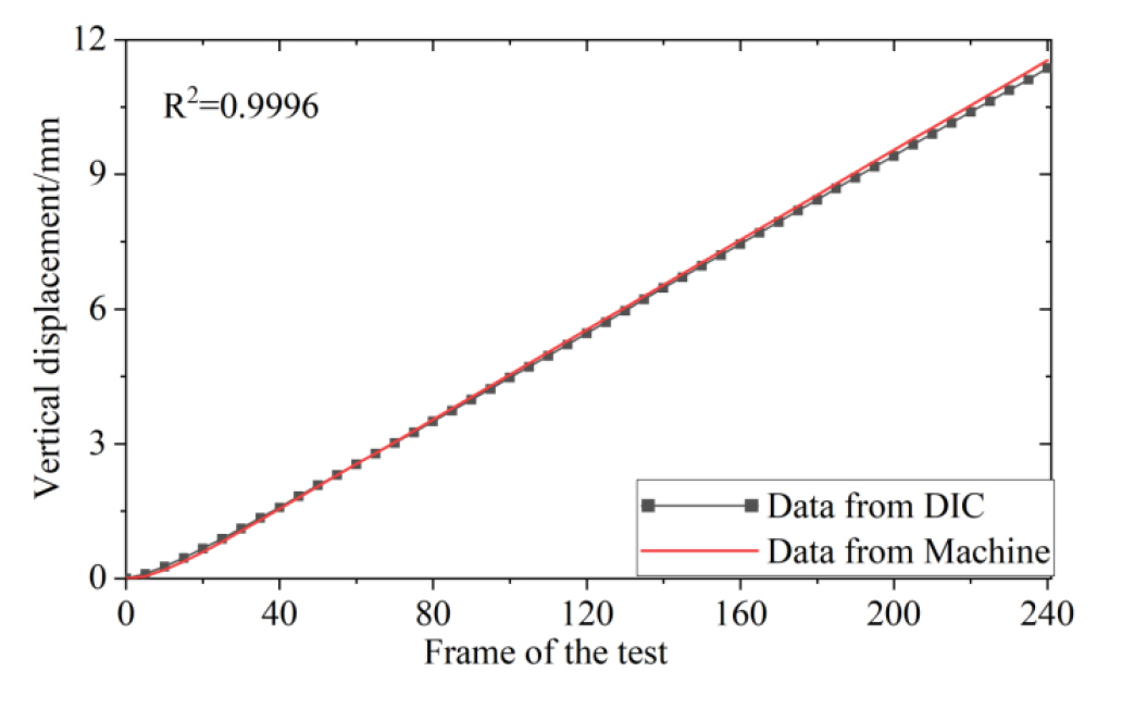
As mentioned previously, the results from a DIC analysis are significantly affected by a number of factors including speckle quality, light intensity, camera noise, among others. Therefore, it is necessary to evaluate the accuracy of DIC results as part of the validation process. Fig. 10 illustrates the accuracy of the DIC results for the footing test. Note here that the horizontal axis (frame of test) indicates a stage of each image taken. The maximum error in terms of the vertical displacement at the location immediately below the footing center between DIC and the actually measured by the machine control system is 0.018 cm, illustrating that the DIC technique can measure soil movement with a high degree of accuracy.
4.2 Soil displacement and strains
VIC-2D, a proprietary DIC software by Correlated Solutions, generates displacements within a designated AOI. For the footing, trapdoor, and retaining wall tests, soil displacements and strains are given below.
4.2.1 Footing test
Table 2 presents the displacement and strain contours, displacement vector plots at different footing load levels. The results show that the DIC well captures the progressive development of displacement and strains as the load level increases. More specifically, the maximum vertical displacement zone appears to develop immediately below the footing, basically moving downward with the footing. With the increase of displacement, the ground on both sides of the footing tends to move upward. In addition, the DIC clearly captures the symmetrically developing radial shear zones that emanate from the edge of the footing. As expected, the radial shear zones gradually expand and then arc-shaped failure surfaces are clearly developed on both sides and extend to the surface.
The footing pressure-settlement curve obtained from the test shown in Fig. 11(a) shows a clearly defined failure point suggesting the general shear failure mechanism Terzaghi theory (Terzaghi, 1943). Such failure mechanics is well illustrated in the failure pattern inferred from the DIC generated major principal strain contours shown in Table 2. For example, a shear failure mechanism is well traced by the DIC, showing a wedge-shaped elastic zone below the footing moving downward and rigid shear zones. Two sliding surfaces are observed, which originate from the footing. The angle between the sliding surface and horizontal angle is related to the internal friction angle of sand. One slide surface originates from the left edge of the footing and reaches the ground on the right side of the footing with the increase of displacement. Similarly, the other slide surface originates with the right edge of the footing and reaches the ground to the left of the footing. The DIC generated results are well in line with the bearing capacity theory (Terzaghi, 1943).
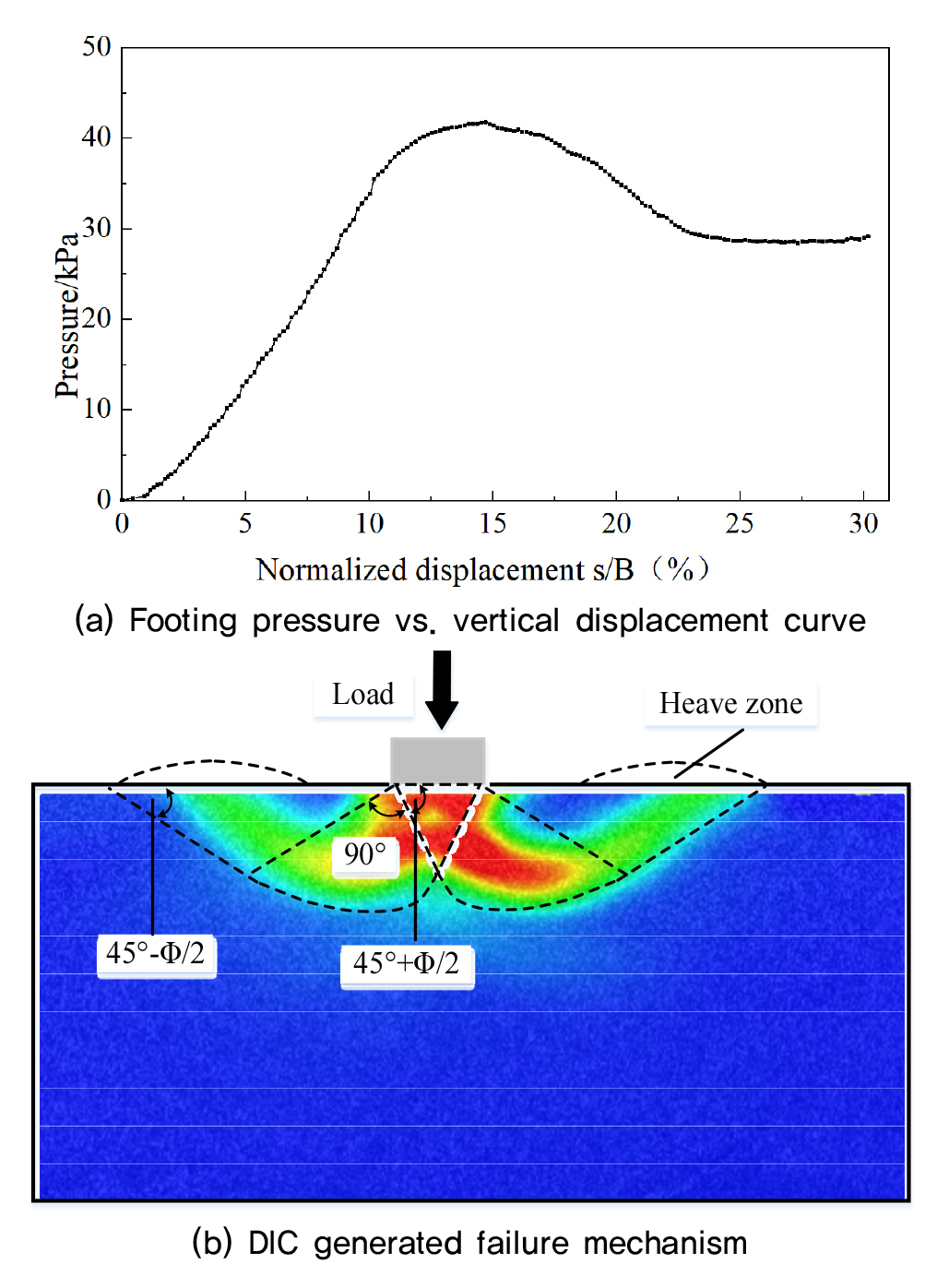
Table 2.
Contour and displacement vector plots for footing test
| State | Pre-failure | Post-failure |
| Vertical displacement | 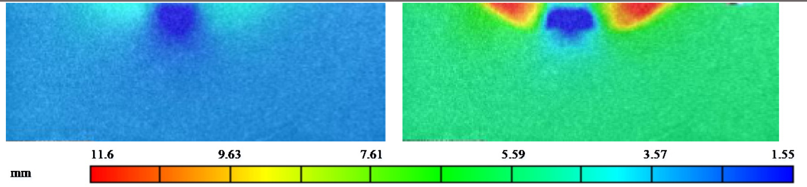 | |
| Major principal strain | 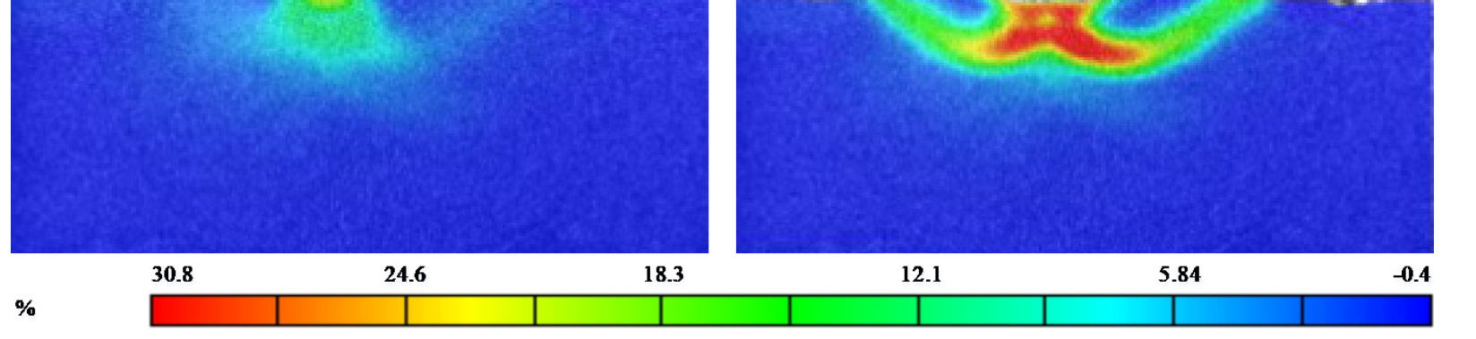 | |
| Displacement vector | 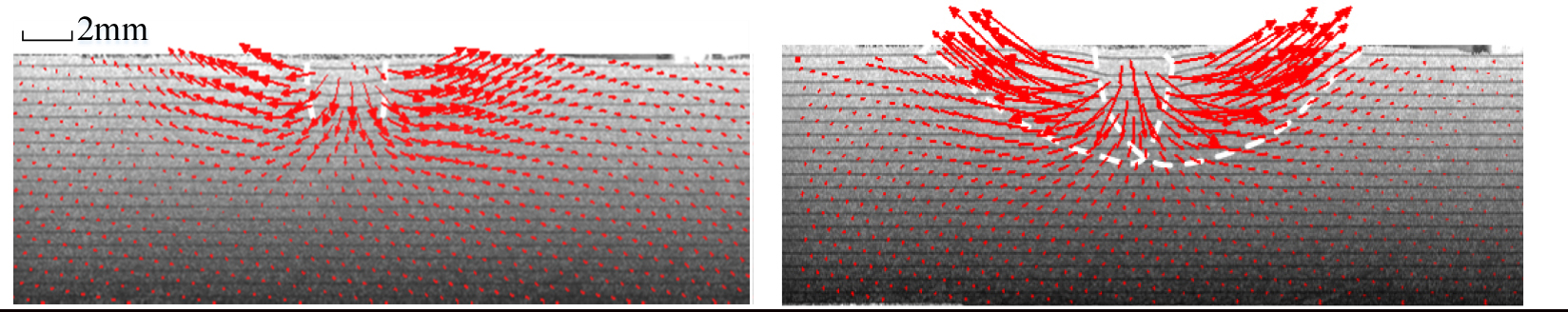 | |
4.2.2 Trapdoor test
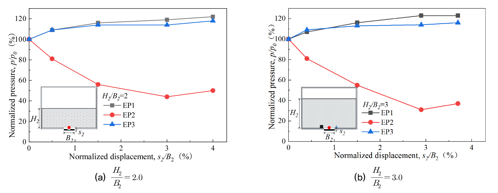
Fig. 12 shows the results of the trapdoor test in terms of vertical pressure versus the vertical displacement of the moving platform. Note that the pressure cells were installed prior to the test during model preparation at the locations shown in Fig. 7. As can be seen in Fig. 12, the load transfer mechanism by arching is clearly demonstrated as the vertical pressure immediately above the moving platform decreases while those at 0.8B2 way from the moving platform slightly increase as the trapdoor moves downward. More specifically for the deep sinkhole case, i.e., , the vertical pressure immediately above the moving platform decreases as great as by 55% from the initial value when the platform moves downward approximately after which the pressure recovers slightly with the continuous downward movement of the platform. On the other hand, the vertical pressures on both sides of the platform slightly increased and then reached stationary values. A similar trend can also be observed in the deep case, i.e., ., as shown in Fig. 12 (a).
These results suggest the formation of arching mechanism as shown in the DIC results in Table 3 where the DIC generated displacement contours and vectors, principal strains are presented. As shown, at the final stage of the trapdoor movement, the DIC generated results well capture the movement of the soil wedge above the trapdoor and the shear plane developed along the lines stretching from the two edges of the trapdoor. The soil movement mechanism is well in line with Terzaghi’s Arching theory as shown in Fig. 13.
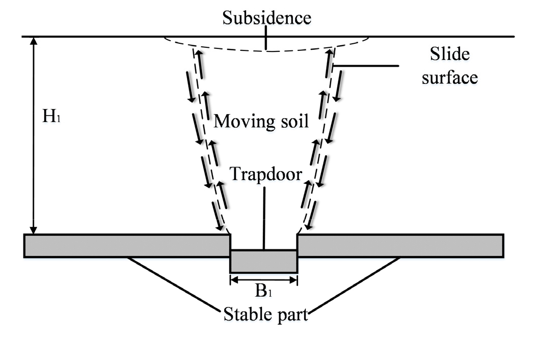
Table 3.
Contour and displacement vector plots from trapdoor test
| Embedment ratios | ||
|
Vertical displacement | 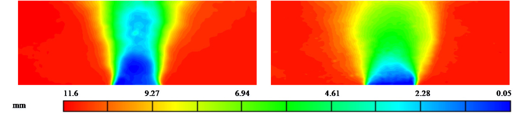 | |
|
Major principal strain | 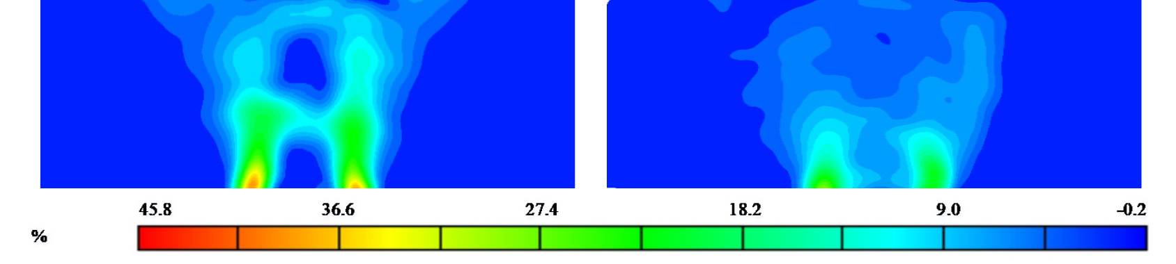 | |
|
Displacement vector | 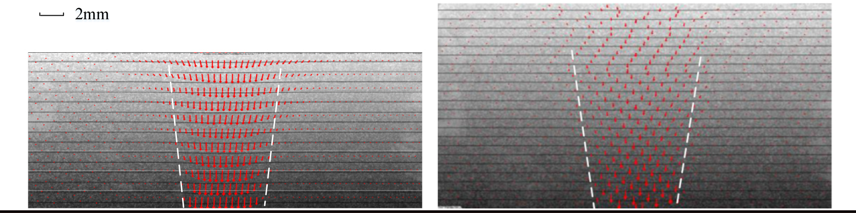 | |
4.2.3 Retaining wall test
Fig. 14 shows the results of the active and passive states in terms of lateral earth pressure versus (σh) the horizontal displacement of the wall (δh). As can be seen in Fig. 14(a) for the active state, the trend of decreasing horizontal earth pressure with increasing the horizontal wall displacement is evident until the horizontal earth pressure (σh) reaches the respective active earth pressure (σa) when . For the passive state, on the other hand, the lateral earth pressures increase with increasing the horizontal wall displacement until reaching the passive earth pressure (σp) when . These results suggest that the retaining wall setup was reasonable to replicate the active and passive state.
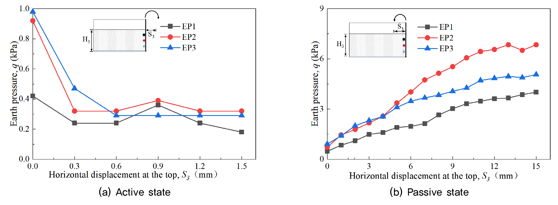
Table 4 shows the displacement and major principal strain contours, displacement vector plots under active and passive states. For the active state, the zone of large horizontal displacement well corresponds to the active failure zone. A close observation reveals that there exist parallel formed active failure lines, which is in line with the classical earth pressure theory. More specifically, a series of parallel straight lines were found to develop where the retaining wall was rotated outward around the toe. Two inclined failure surfaces were observed, which is consistent with the test results of Niedostatkiewicz et al. (2011). The active failure surface can also be inferred from the major principal strain contour plot shown in Table 4, where the angle between the failure surface and the soil surface was observed to be approximately 56° which is in good agreement with the Rankine active failure surface angle with .
Table 4.
Contour and displacement vector plots for retaining wall test (wall rotation angle 15°)
| Load state | Active state | Passive state |
|
Vertical displacement | 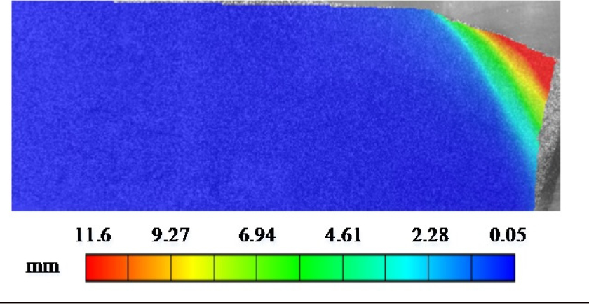 | 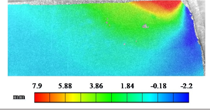 |
|
Major principal strain | 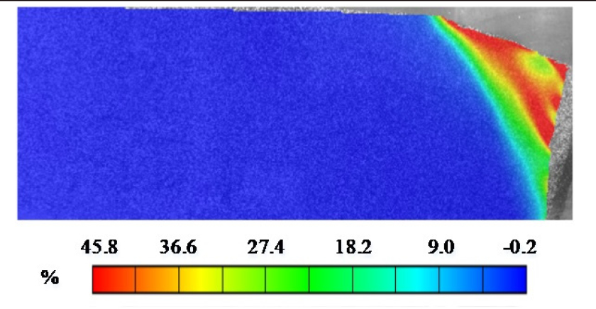 | 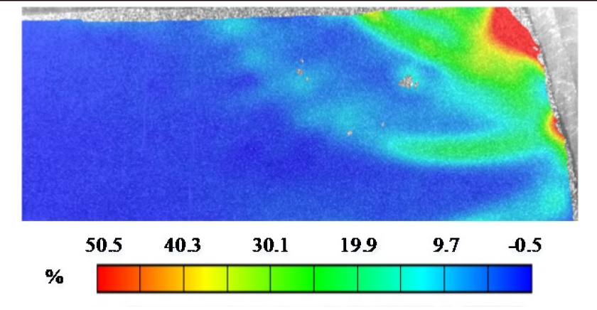 |
|
Displacement vector | 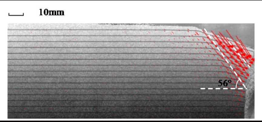 | 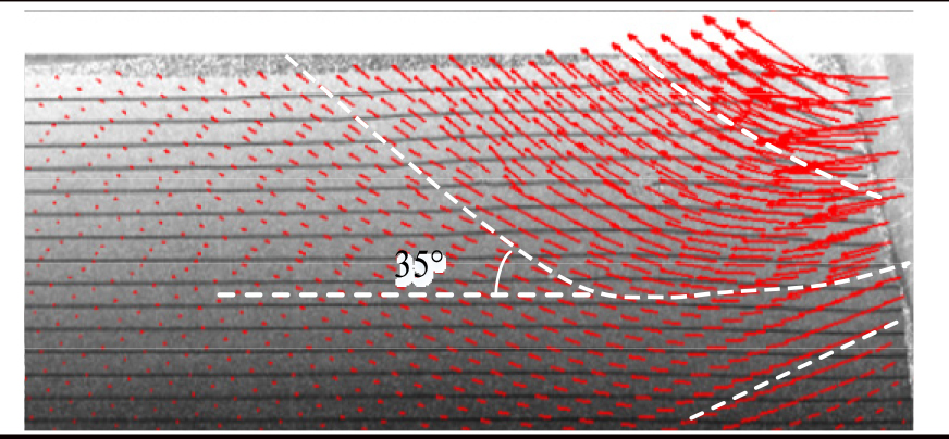 |
Different from the active state, the range of displacement region is wider in the passive state as shown in Table 4. The maximum principal strain contour plot also shows a wide zone of the plastic zone with a curved failure surface. A maximum principal strain zone is observed at the top of the retaining plate, and the range of the region gradually expands with the increase of rotation angle. Two curve failure surfaces with similar shapes propagate in the soil. They originate from the retaining wall, one extends to the surface, and the lower one extends downward to the bottom. This is similar to the observation of Bransby (1968). However, in this test, the lowest failure surface in the soil did not extend to the surface. The observed failure pattern is somewhat different from the horizontal straight line of surface assumed in the Rankine active earth pressure theory. The angle of passive state failure surface, θp = 35°, seems to be a bit larger than the Rankine passive earth pressure theory, . These results suggest that the DIC technic can be effectively used in identifying failure mechanisms of geo-structures.
4.3 Geogrid strains
Fig. 15 illustrates the force-time curve obtained from a wide stretch test of a geogrid. As can be seen from the graph, the force increases slowly at the beginning due to the relaxation behavior and then varies linearly with time. The force reached 10 kN/m at the seventh second and the ribs broke at approximately fourteenth seconds with a breaking force of 20 kN/m.
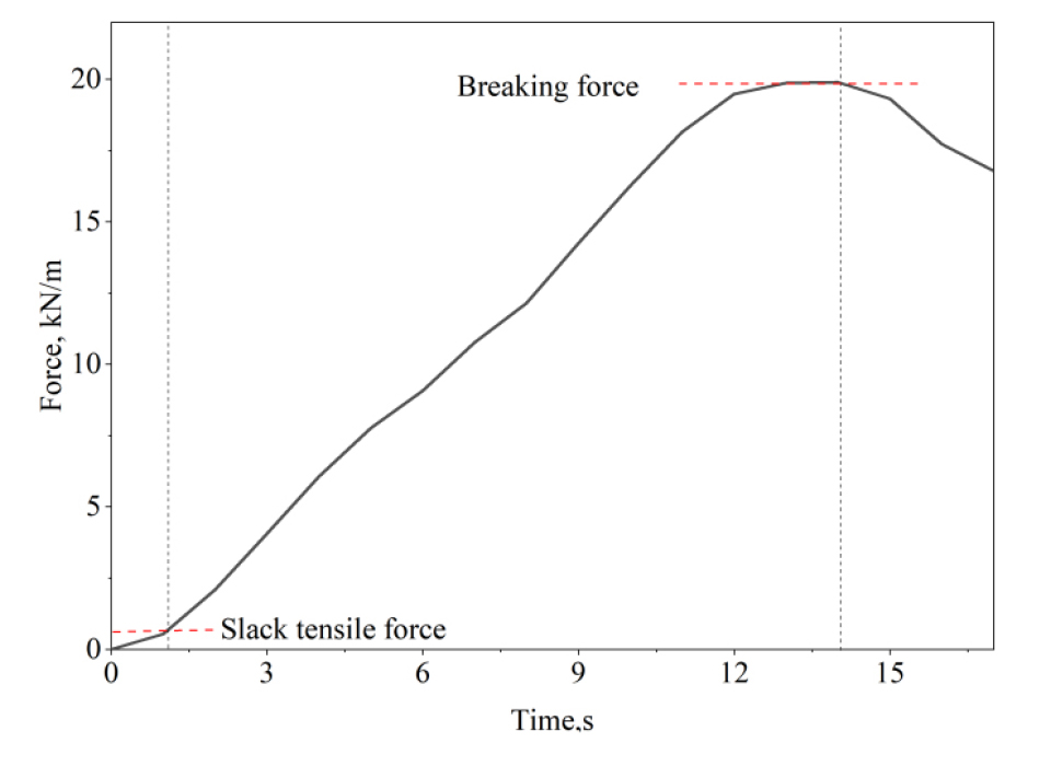
Table 5 shows the vertical displacement and vertical strain contour plots for the geogrid at different moments. The vertical displacements are distributed in a gradient, with the lowest part of the specimen showing the smallest displacements and the uppermost part showing the largest displacements as the clamp moves upwards. Based on the results of the vertical strains, it can be seen that the distribution of strains in the geogrid during tension is not uniform, with the vertical ribs experiencing large tensile strains and the transverse ribs having nearly zero strain. As the rib in the middle of the specimen slides slightly out of the fixture during tension, the strain on the middle rib is significantly less than the strain on the ribs on either side. Some parts of the geogrid are at extremely high strains, with a maximum strain value of 9.69%, due to defective errors in the fabrication process of the geogrid.
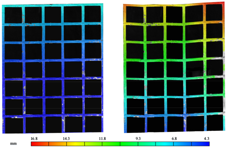
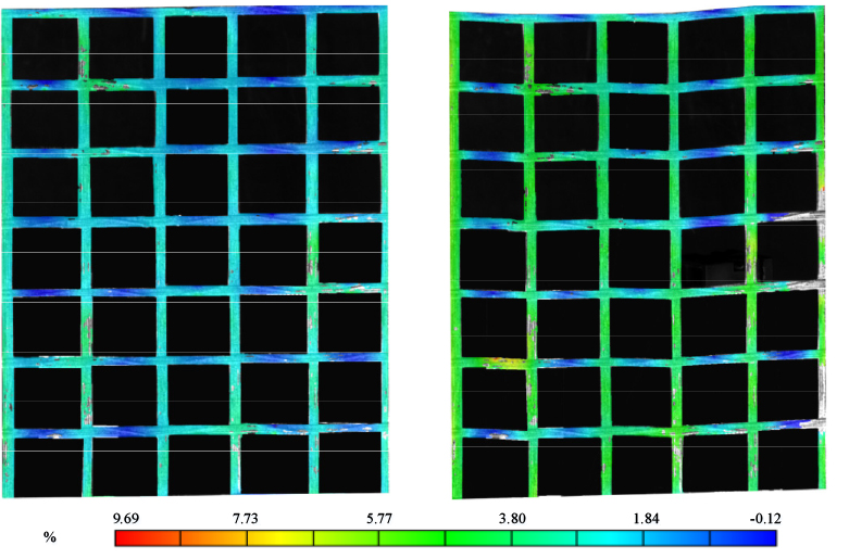
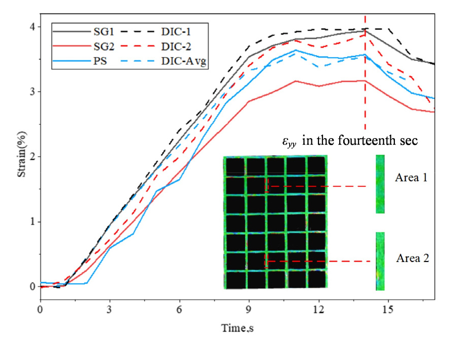
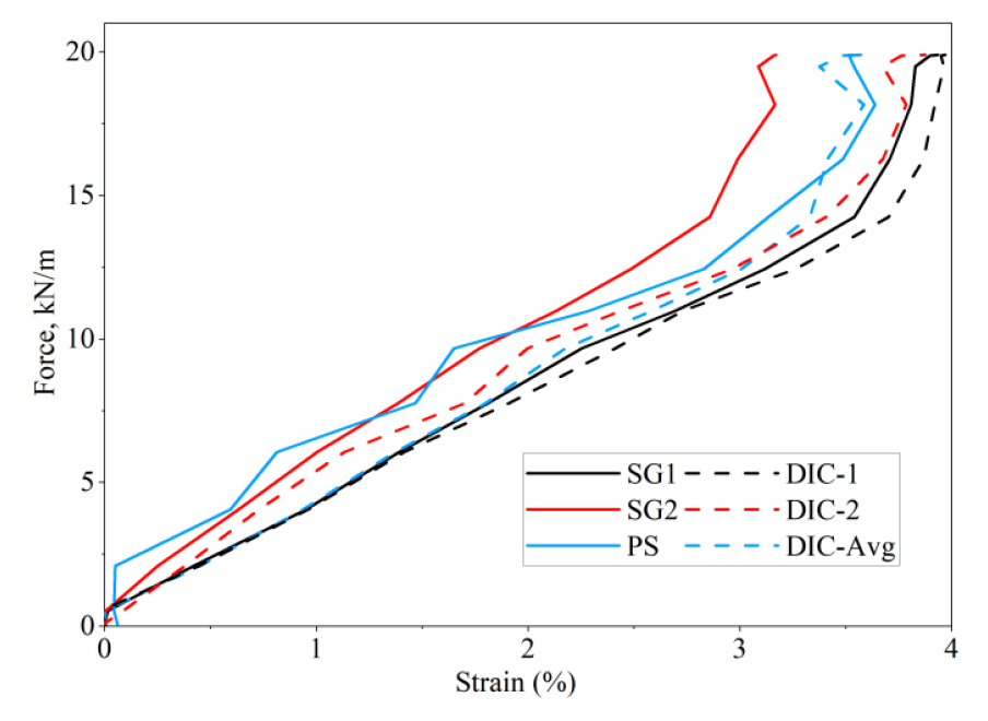
Fig. 16 compares the average and local strains obtained by the different methods. It can be seen that the average strain obtained from the position sensor and the DIC is approximately 3.5%, with the change in the position sensor slightly lagging behind the change in the DIC. The locations where the strain gauges were attached were area 1 and area 2, respectively. For verification purposes, area 1, 2 was selected in the strain contour using the DIC plotting tool, and the local strain is slightly greater than the average strain value, which is approximately 3.9%. Strain gauge 2 was partially dislodged during the tensile test, resulting in a final strain value of 3.2%, resulting in a relatively small strain value, which is a limitation of the conventional method. Fig. 17 shows a graph of the force versus strain curve from the start to the breakage of the geogrid, plotted according to the different methods (strain gauges, position sensors, DIC) tested during the test. The force varies linearly with strain, with a breaking force of 20 kN/m when the strain reaches approximately 3.5%. As can be seen from the results in Fig. 17, both the DIC and the correctly installed sensors are able to obtain accurate strains.
Through the results above, it is clear that the results using the sensor and DIC measurements are highly consistent. These test results, therefore, show that DIC technology can not only acquire full-field deformations but can also be effectively used for local strain measurements in geosynthetics, which is a major advantage over conventional monitoring methods.
5. Conclusions
In this paper, the use application of advanced digital image correlation (DIC) technology in the geotechnical tests is examined, such as shallow footing bearing capacity test, trapdoor test, retaining wall test, and wide width tensile test on geogrid. Theoretical background of the DIC technique is first introduced together with fundamental equations. Relevant reduced-scale model tests were then performed using standard sand while applying the DIC technique to capture the target material point movement. The results of the tests were carefully analyzed using the displacement contours and vector plot, strain contour plots together with measured values by conventional monitoring instruments. The results show that the DIC technique can be effectively utilized in reduced-scale geotechnical tests in closely tracing material points movements and trace potential failure mechanisms. Together with a proprietary DIC software, it was possible to calculate strains developed in soil within the AOI as routine outputs. Such capability of the DIC technique has can open the door for more advanced analysis of macro scale material points movements which will hopefully allow a better understanding of mechanistic behavior of material under various loading conditions.
It is also shown that the complete displacement and strain field of sand in the whole process are obtained by DIC technology, which can not only directly reflect the generation, expansion, and interconnected evolution process of failure surface but also determine the specific information such as the shape and expansion direction of the failure surface. Compared with traditional test methods, it has obvious advantages and provides an effective means for studying the macro and micro deformation and failure mechanism of rock and soil, This is of great significance for the in-depth study of the failure mechanism of geotechnical tests.
