1. Introduction

The use of EPS geofoam as a subgrade in road construction might be an alternative method to poor bearing capacity soils because the unit weight of EPS geofoam is just 0.3 kN/m³, nearly equivalent to 15~30 of that of most natural soils. It was noted that the first application of EPS geofoam was performed for the road frost protection purposes in Norway. Since 1972, research studies on EPS geofoam have been achieved in many types of civil engineering applications. However, it was observed that no standard method of resilient modulus test on EPS geofoam was reported. Instead, some papers and reference books (Stark et al, 2004; Horvath, 1995) introduced the calculated resilient modulus of EPS geofoam based on California Bearing Ratio (CBR) and R-value, or EPS geofoam Young’s modulus was directly used as resilient modulus. In a current trend of pavement design, the resilient modulus is one of most important input parameters as it is the dynamic response to a moving wheel loading. It should be noted that the Young’s modulus of EPS geofoam is obtained from static response to a static load. Thus, resilient modulus and Young’s modulus of a subgrade material have an apparently different principle according to applied stress conditions. In order to execute a proper pavement design, the resilient modulus from dynamic experimental testing is necessary for better performance in road construction using EPS geofoam as a subgrade.

2. Triaxial Compression Tests

2.1 Experimental Parameters

The selection of the experimental parameters was very important task to investigate, estimate, and analyze the test results for the desired purpose of those works. Thus, in this study, the experimental parameters were chosen based on the purpose of obtaining resilient modulus. Characteristic of resilient modulus of EPS geofoam is dependent on several parameters such as unit weight, stress conditions, number of load repetitions, moisture, and temperature (Myhre, 1995). Moisture and temperature were not considered in this study since these parameters had little effects on resilient modulus compared to other parameters for use of EPS geofoam material. Therefore, the experimental program has been established to study a relationship among cyclic stress, unit weight, and number of load repetitions.

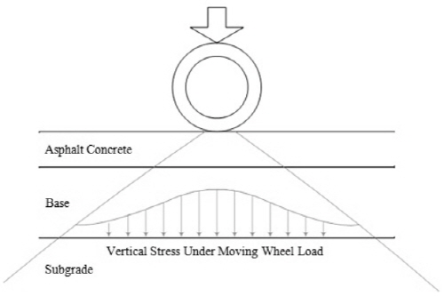
The above stress parameters were considered to be those that would be simulated according to the stress ranges of a subgrade layer below pavement structures in-situ. The stress pulse time can be related to the vehicle speed and depth as shown in Fig. 1. The loading time is based on the average pulse time for stresses in the vertical and horizontal directions at various depths. When the elastic theory is employed to analyze pavements, the duration of loading for determining the resilient modulus under repeated loading can be 0.1 second of loading and a rest period of 0.9 second with a haversine load (Huang, 1993).

2.2 Test Results

An already existing standard methodology to determine the resilient modulus of subgrade soil was investigated for its suitability regarding EPS geofoam because there was no specified method for resilient modulus of EPS geofoam. The triaxial compression testing was conducted by utilizing MTS 858 Mini Bionix II composed of triaxial chamber, load cell, air pressure regulator, digital air pressure gauge and Hydraulic Power Unit. In order to complete this task, the resilient modulus from experimental tests were compared at 100th, 5000th, and 10000th cycle of load repetitions including the unit weights of 0.24 kN/m³, 0.31 kN/m³, and 0.47 kN/m³.

Fig. 2 shows representative test results with a 60kPa deviator stress and 62.1kPa confining stress with unit weights of 0.24 kN/m³, 0.31kN/m³, and 0.47 kN/m³. Fig. 2 indicates that the resilient modulus can be explicitly classified by unit weights of EPS geofoam and considered as a function of materials’ unit weights as well. However, there are no significant differences among their magnitudes along the same unit weight at 100th, 500th, 1000th, and 10000th cycle. In fact, the rates of difference are 1.1% between 100 and 10,000 cycles for 0.24 kN/m³, 13.4% for 0.31 kN/m³, and 5.1% for 0.47 kN/m³. In 0.31 kN/m³, a rate of difference between 500th and 10000th cycle is just 1.3%, which means the resilient modulus at the 100th cycle may include somewhat uncertain errors from measuring and preparing the specimen. Therefore, as the results of analytical analysis, it was noted that the resilient modulus method from AASHTO T307 was applicable for EPS geofoam as a subgrade material, in practice, which was concluded by analyses of all test results with a combination of all 27 types testing conditions as mentioned previously (AASHTO, 2003).

2.3 Resilient Modulus

It is necessary that the mechanical properties of the resilient behaviors need to be determined over a certain number of repeated applications where the resilient strain becomes constant. The resilient modulus is defined as the ratio of the applied deviator stress to the recoverable axial strain (Huang, 1993).

 = /                                    (1)

where,  : resilient modulus  : axial deviator stress : axial recoverable strain

There are two components to the total deformation, a resilient (recoverable) portion and a plastic (permanent) portion. Only the resilient portion is included in the measurement of resilient modulus. This resilient strain can be obtained when the increment of the plastic strain is completed and the specimen gets a steady state after approximately 1000th cycle in the tests of this study.

3. Analytical Works

3.1 RMEG Program

2-dimensional plane strain finite element analysis was carried out to investigate a typical highway cross-section by using RMEG program written in FORTRAN 90 which was modified based on 2DFEM program developed by Professor Sangchul Bang of SDSM&T (Bang, 1995). Several subroutines in RMEG program were adopted from the original finite element analysis program, 2DFEM. RMEG program has a main body including several subroutines such as RMEPS, CSOLVE, BECOL, QUAD, FORMB, DUNT, and PRST. This program uses an open statement data input system. The subroutine RMEPS calculates resilient modulus of EPS subgrade using its model which needs parameters such as deviator stress, confining stress, and unit weight. The subroutine CSOLVE solves the sim-ultaneous equations by gauss elimination. The BECOL calculates the element stiffness matrices and load vectors and recovers the element strains and forces of beam- column elements. The subroutine QUAD calculates the element stiffness matrices and load vectors and recovers the element strains and stresses of 4-nodal quadrilateral element. The subroutine FORMB calculates ‘B’ matrix of 4-nodal quadrilateral element. The subroutine DUNT calculates the continuum modulus and Poisson’s ratio by modified Duncan’s hyperbolic model. The subroutine PRST calculates the principal stresses.

3.2 Resilient Modulus Model of EPS Geofoam

For the subgrade soils, there are many available pre-diction models or constitutive equations of the resilient modulus from various public materials. However, no papers were found for the resilient modulus model of EPS geofoam. Developing the resilient modulus model of EPS geofoam is essential in highway engineering practice using EPS geofoam as a subgrade material to accomplish successful pavement design without distresses on pavement surface over poor bearing capacity soils. Analytical works were performed by conducting linear regressions on the results of long-term repeated load triaxial compression tests. During this project, more than 54 EPS geofoam of cylindrical specimens having 101.6 mm of diameter and 203.2 mm of height were used. The average values of all tests results were obtained and analyzed to produce rational test data yielding proper resilient modulus values based on given testing conditions. That is why all specimens that resulted in irrational and meaningless test results were discarded and retested for those conditions.

3.3 Development of Resilient Modulus Model of EPS Geofoam

Based on the measured resilient modulus values in Table 2, regression analyses were conducted to develop mathematical equations incorporating all 54 measured data points by using the concept that M_R is a function of deviator stress, confining stress and unit weight of EPS geofoam. Once this mathematical model is developed, it is possible for a pavement designer to predict a resilient modulus with any conditions of stresses and densities of EPS geofoam by using the following model with unit weight limits of (13 kPa ≤ ≤ 70 kPa) for unit weight of 0.24 kN/m³, (13 kPa ≤ ≤ 90 kPa) for [0.31 kN/m³ unit weight 0.47 kN/m³], (13 kPa ≤ ≤ 70 kPa) and (0.24 kN/m³ ≤ ≤ 0.47 kN/m³).

It is noted that the dependent variable, M_R, is a function of deviator stress, confining stress, and unit weight as mentioned previously. Therefore, a mathematical model should comprise all three factors as independent variables on it. The proposed basic equation is below

 (2)

where, X : deviator stressY : confining stressZ : unit weight of EPS geofoam

k₁, k₂, k₃, and k₄ : regression constants

The result of regression analysis has a good agreement with 0.96 of R-square. The outputs of analysis were

      k₁  = 1.4820

      k₂  = -0.0813

      k₃  = 0.0707

      k₄  = 0.4105

Then, Eq. 1 can be expressed with the found co-efficients as follows

 (3)

where,  : deviator stress : confining stress : unit weight of EPS geofoam

The range of stress and unit weight should be limited on the analytical model as follows :

      (13 kPa ≤ ≤ 70 kPa) for unit weight of 0.24 kN/m³

      (13 kPa ≤ ≤ 90 kPa) for [0.31 kN/m³ ≤ unit weight ≤ 0.47 kN/m³]

      (13 kPa ≤ ≤ 70 kPa) for unit weight of 0.24 kN/m³ or higher

      (0.24 kN/m³ ≤ ≤ 0.47 kN/m³)

These ranges are in accordance with the elastic limit stress of EPS geofoam (Stark et al, 2004).

4. Finite Element Analysis

4.1 Assumption of Modeling

The concept of the plane strain in geotechnical engin-eering practice is to take advantage of geotechnical in-situ conditions having infinitely long dimensions along the z-direction with no strain (ε_z=0) out-of-plane x-y (Ugural et al, 1995). Therefore, there is no need to carry out a full 3-dimensional stress analysis, i.e., a real 3-D problem can be reduced to a 2-D problem and a linear elastic multi-layer system can be considered to design the flexible pavement with RMEG FORTRAN program.

4.2 Modeled Traction Pressure

The modeled traction pressure corresponds to 707 kPa, which is a standard representative contact stresses in modeling flexible pavement analysis. The representative contact stress of 707 kPa was applied on the upper element.

4.3 Finite Element Mesh

In the FEM analysis, a typical flexible pavement cross- section was adopted. The typical flexible pavement structure with EPS subgrade consists of asphalt pavement with 101.7 mm, base of crushed rock with 203.2 mm, subbase of open-aggregate with 203.2 mm, sand with 152.4 mm, concrete capping slab with 45.7 mm, and EPS subgrade with 304.8 mm. The mesh consists of 99 nodes and 80 elements. The concept of symmetry is used in developing the 2-D FEM mesh because the loading configuration and the mesh geometry are symmetric in the transverse direction and is the same along the longitudinal direction, so it can be reduced to a two dimensional plane strain problem without any significant effect. Elements were numbered left to right and bottom to top. The elements 73 through 80 were assigned for the pavement elements and the elements 57 through 72 were assigned for the base elements with two layers. The elements 41 through 56 were assigned for the subbase elements and the elements 33 through 40 were assigned for the capping layer for the EPS subgrade. The elements 1 through 32 were assigned for the EPS subgrade begun from the bottom of the pavement structure. The 538 kPa and 861 kPa wheel loadings were applied between node 11 and node 22 on element 73.

5. Design Equations of Flexible Pavement

The AASHTO developed the concept of incorporating a reliability factors into the design procedures to ensure that the various alternatives would allow for inherent design and construction variability and perform as they were intended in the design period. Modified design equation for flexible pavement was represented in 1993 as follows (AASHTO, 1993)

   (4)

where, W₁₈ : predicted number of 18-kip equivalent single axle load applications

Z_R : standard normal deviate

S_o : combined standard error of the traffic prediction and performance prediction

ΔPSI : difference between the initial design serviceability index, p_o, and the design terminal serviceability index, p_t

M_R : resilient modulus of subgrade material (psi)

SN : structural number of pavement

 (5)

a_i  : ith layer coefficient

D_i : ith layer thickness (inch)

M_i : ith layer drainage coefficient

In Eq. 3, W₁₈ includes traffic information required and represents that a standard 18-kip (80.1-kN)-equivalent single-axle load (ESAL). In other words, the damaging effect of the passage of an axle of any load can be represented by a number of 18-kip equivalent single axle loads. For instance, one application of a 12-kip single axle was found to cause damage equal to approximately 0.23 applications of an 18-kip single axle load, thus four applications of a 12-kip single axle were required to cause the same damage as one application of an 18-kip single axle (Mannering et al, 1998).

6. Case Studies

This section has two main parts. One is using RMEG Fortran program to analyze the flexible pavement with given conditions and the second part is to apply the AASHTO flexible pavement design method to estimate a design life with a certain desired confidence. The typical highway cross-section was investigated using the modified computer program (RMEG). The vertical displacements and compressive stress were obtained and analyzed. In this study, a linear elastic multi-layer system was used. All material properties used are shown in Table 3.

6.1 Prediction of Deformaion

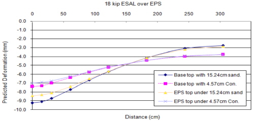
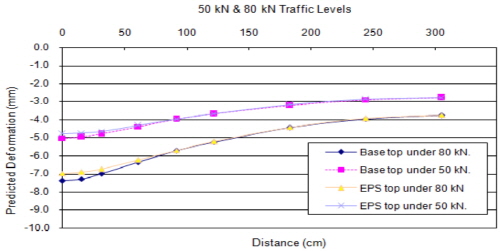
Fig. 4 shows the vertical displacements on the underlying pavement layers and on overlying EPS geofoam layers. Fig. 4 indicates that the deformations of two types of pavement structures with 152.4 mm sand capping and 45.7 mm concrete slab capping have only less than 2.54 mm different deformation. Consequently, for the EPS geofoam as subgrade, it could be recommended to use 45.7 mm concrete slab capping rather than 152.4 mm sand layer. The deformation of the pavement structure with concrete slab capping shows approximately 2.54 mm less than that of sand capping. Fig. 5 shows the comparison of deformation with 50 kN and 80 kN of vehicle loads indicating the pavement structure under 50 kN of vehicle load experiences 30 % less deformation. Fig. 6 represents the deformations with three types of EPS unit weights under 80 kN traffic load. As seen in the Fig. 6 the higher density experiences less deformation.

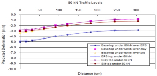
Comparing curves on Fig. 7 indicates that the pavement structures of silt, clay, and EPS geofoam based subgrades deform closely under 50 kN traffic load. This means the use of EPS geofoam material as a subgrade is suitable for the road construction over the weak and compressible soils having low bearing capacity. Furthermore, these types of soft soils may exceed the limit of the settlement with a long period time, whereas EPS blocks do not consolidate significantly with a long period time. As shown in Fig. 7, 0.31 kN/m³ EPS block shows almost same deformation behaviors with silt 18.9 kN/m³ and clay 16.5 kN/m³ by less than 0.254 cm.

6.2 AASHTO Flexible Pavement Design

Through this procedure, the pre-mentioned FEM analysis on deformation can be utilized to predict how long the deformation of pavement structure will last without a great severe distress on the pavement. For this examination, the following are assumed as daily traffic conditions on the highway with 70% r eliability. According to NCHRP REPORT 529, the EPS geofoam is recommended to be used for low volume traffic levels meaning 50%∼75% reliability level. Thus, in this case study, the reliability level is set as 70% (Stark et al, 2004).

Assuming the design daily traffic and other necessary indexes are as follows (Mannering et al, 1998) :

      189  20-kip (89.0-kN)  : single axles

      70   24-kip (106.8-kN) : single axles

      119  40-kip (177.9-kN) : tandem axles

      R : 70% (Z_R = -0.524)

      ΔPSI : 2.2 (PSI – TSI)

structural-layer coefficients are :

      Hot-mix asphaltic concrete :       0.44

      Emulsion-bituminous :             0.30

      Crushed stone :                  0.11

      Reinforce concrete slab :  0.5

      a₁ = 0.44, a₂ = 0.3, a₃ = 0.11, a₄ = 0.5

The following are the thickness of the pavement materials used in design:

      Asphalt concrete as wearing surface : 101.7 mm

      Crushed stone as base layer : 203.2 mm

      Open aggregate as subbase layer : 203.2 mm

      Concrete slab capping layer : 45.7 mm

Substituting all parameters into Eq. 4,

      5.94 = 0.44(4.0) + 0.30(8.0)(1.0) + 0.11(8.0)(1.0) + 0.5(1.8)(1.0)

      20-kip (89.0-kN) : single axles equivalent = 1.51

      24-kip (106.8-kN) : single axles equivalent = 3.03

      40-kip (177.9-kN) : tandem axles equivalent = 2.08

Thus total daily 18-kip ESAL is

      Daily W₁₈ = 1.51(189) + 3.03(70) + 2.08(119)

               = 745.01 (18-kip ESAL)

Converting Daily W₁₈, W₁₈ is 5,601,730. This results in

This indicates that 18-kip of vehicle load passes 500 times a day and the pavement will last at least 20.6 years without significant distresses.

6.3 Results of Case Studies

As mentioned previously, the AASHTO flexible pavement design procedure with assumed conditions can expect the design life with desired confidence level such as 50%∼75% reliability which are the recommended reliability levels on EPS geofoam for low-volume road design. All given conditions were substituted into Eq. 3 with 4.57 cm concrete slab and 13 MPa resilient modulus of EPS geofoam. The calculation shows that this pavement structure would last at least 20.6 years. In addition to this expectation, the RMEG program has shown in Fig. 6 that this pavement structure will experience less than 5 mm deformation with 70% reliability during 20.6 years. But no statement is available for distresses on the pavement surface in this analysis, because the problem of distresses such as rutting and cracking is another material problem, i.e., asphalt concrete. This study focused on the de-formation caused by subgrade material with the resilient modulus model of EPS geofoam.

7. Conclusion

The use of Expanded Polystyrene (EPS) geofoam as a subgrade in road construction is an alternative method to support loads induced by traffic vehicles over weak, poor, and compressible subgrde soils. Through the experimental tests, finite element analysis, and AASHTO flexible pave-ment design method, it was considered that the EPS geofoam was proper material as a subgrade in the flexible pavement.

The finite element analysis and AASHTO flexible pave-ment design method provided the predicted deformation of the desired type of flexible pavement structure and the design life of the pavement structure. It should be noted that in pavement design, most concerns are about how long it would last without a severe distress on the pave-ment surface and how big the magnitude of deformation would occur during the desired design life. These two fundamental concerns can be solved with the RMEG FORTRAN program and the AASHTO flexible pavement design method using the analytical prediction model for the resilient modulus of EPS geofoam developed in this study.