

1. 서 론
2. Manzari-Dafalias 모델
2.1 Yield criteria in 3-D stress space and flow rule
2.2 Critical, dilatancy, and bounding surfaces in 3-D stress space
2.3 Isotropic and kinematic hardening
2.4 Dilatancy coefficient D
2.5 Hypoelasticity
2.6 한계상태
3. MD 모델 파라미터
4. MD 모델 파라미터 민감도 분석
4.1 곡면 파라미터
4.2 항복곡면 파라미터 , 등방경화 파라미터 , 이동경화 파라미터
4.3 Dilation 파라미터
4. 결 론
1. 서 론
조립재료 중에서 자갈은 토목 및 건축 분야에 있어서 널리 사용되는 재료로서 대표적으로 댐제방, 철도 하부지반, 옹벽 및 교량 교각의 뒤채움 재료로서 활용되고 있다. 자갈재료의 공학적 거동은 모래의 거동과 유사한 것으로 알려져 있으나, 자갈은 전단하중을 받을 경우 모래와 비교하여 입자간의 팽창이 보다 많이 발생하고 이에 따라 음의 간극수압이 크게 발생하는 것으로 알려져 있다(Taylor et al., 1995). 이러한 자갈재료의 거동을 예측하고 수치해석적으로 분석하기 위해서는 자갈재료의 구성모델이 필요하며 다수의 모델이 제시되어 왔다(Prevost, 1985; Banerjee et al., 1992; Dafalias, 1986; Manzari and Dafalias, 1997). 조립재료에 대한 다수의 구성모델 중에서 Manzari and Dafalias(1997) 모델은 조립재료의 상태 및 배수조건에 따라 경화 및 연화 현상을 모사할 수 있는 특징을 가지고 있으며, 한 세트의 모델 정수를 활용하여, 배수 조건, 구속압, 간극비에 상관없이 조립재료의 거동을 구현할 수 있는 장점을 지니고 있다. 조립재료의 거동을 예측하기 위해서 구성모델이 모사해야할 가장 큰 특징은 응력에 따른 팽창(stress-dilatancy), 응력의 방향이 변화할 때 간극수압의 변화 예측, 응력 경로에 따른 재료 거동 특성 등이며 Manzari and Dafalias(1997) 모델은 이러한 거동 양상을 정성적으로 예측할 수 있다.
하지만, 구성모델을 정확히 활용하기 위해서는 개발된 모델을 정의하는 각각의 파라미터들의 역할을 명확히 이해하여야 하며, 각 파라미터의 변화가 재료의 해석에 미치는 영향을 사전에 이해하고 있어야 한다. 본 논문에서는 Manzari and Dafalias(1997) 모델을 구성하는 각각의 파라미터에 대하여 분석하며, 또한 민감도 분석을 통해 파라미터들이 재료의 역학적 거동에 미치는 영향을 제시하고자 한다.
2. Manzari-Dafalias 모델
본 절에서는 한계상태 및 bounding surface soil plasticity 이론을 기본개념으로 개발된 MD(Manzari-Dafalias) 모델의 구성에 대하여 설명한다. MD모델의 기본 개념은 소성계수(plastic modulus)를 찾는데 있어서 현재 응력상태(current state of stress)와 bounding surface에 투영된 이미지 응력상태(image state of stress)간의 거리를 활용하며, 한계상태 개념하에 상태 변수인  를 활용하여 체적변형을 예측하고 응력-변형률 관계를 모사한다. 여기서,
  와
와  는 각각 토사의 간극비와 한계상태 간극비를 나타낸다. 모델 내에서 bounding surface 개념은 축차응력비 공간(deviatoric stress-ratio space)에서 이미지 응력상태를 추정하는 역할을 수행하고, 상태변수
  는 조립재료의 체적변형 거동을 규명하는 역할을 수행한다.
MD모델은 토사의 상태 및 배수조건에 따라 경화 및 연화현상을 모사할 수 있는 특징을 가지고 있으며, 한 세트의 모델 정수를 활용하여, 배수 조건, 구속압, 간극비에 상관없이 조립재료의 거동을 구현할 수 있는 장점을 지니고 있다. 모델에 관한 자세한 사항은 Manzari and Dafalias (1997), Manzari and Prachathananukit(2001), Choi(2004)를 참조한다.
본 절에서는 MD모델에 대한 개념적 정의를 제시하며, 다음의 설명에서 압축응력 및 변형이 양(+)의 값을 나타내고, 볼드폰트는 텐서량을 표현하는데 사용된다. Table 1은 본 논문에서 사용되는 응력과 변형률 텐서에 관한 표현 및 정의를 보여준다.
Table 1. Representation of stress and strain | ||
Stress Representation | Strain Representation | Other Notations |
|
|
|
|
| |
|
| |
|
| |

 : pore water pressure increment


2.1 Yield criteria in 3-D stress space and flow rule
MD모델의 항복곡면은 응력비공간(stress ratio space)에서 쐐기형태로 표현된다. 즉, 항복곡면은 정점이 원점에 위치한 원뿔꼴로 식(1)과 같이 표현된다.
(1)
여기서,  은 식(2)와 같고
  은 식(3)과 같다.
(2)
(3)
 은 축차평면상의 응력텐서이며
  은 norm을 의미한다. 축차 대비응력비(back-stress ratio) 텐서
  와 응력비 스칼라 m은 각각 항복곡면의 이동경화(kinematic hardening)와 등방경화(isotropic hardening)를 정의한다. 항복곡면을
  의 축차응력평면으로 투영하면 Fig. 1에서와 같은 원형 모양으로 나타난다. 식 (1)의 항복함수를
 ,
,  , and
, and  as related to
  ,
,  , and Lode angle
  (modified after Manzari and Dafalias, 1997).
주응력공간에서 표현하면 Fig. 2에서와 같이 반지름이
|
Fig. 2. Schematic view of circular yield surface in three dimensional principal stress space : |
 and
and  denote elastic domain and elastic yielding boundary, respectively (Choi, 2004).
 이고 중심이
  인 원점에 정점이 위치한 원뿔꼴로
묘사된다.
식 (1)에서 나타난 바와 같이 항복함수는 등방정적축(hydrostatic axis)을 따라 열려 있으므로, MD모델은 순수 체적항복(pure volumetric yielding)을 정의하지 않음을 알 수 있다. 응력 공간내에서 항복함수에 대한 수직(normal)  과 소성변형의 방향
  은 식 (4)와 식 (5)로 정의된다.
(4)
(5)
여기서,  ,
,  ,
,  , 1 은 각각 식(6), 식(7)과 같다.
(6)
(7)
D = dilatancy coefficient
1 = 2nd order identity tensor
 은 단위 축차 응력비 텐서를 나타내며,
  과
과  의 특성을 지닌다. 식 (4)와 식 (5)로부터
  은 항복곡면에 수직인 함수를 나타내고,
  은 소성변형율 텐서의 방향을 결정한다. 식 (4)와 식 (5)의 공통적인 요소인
  은 축차응력비 공간에서는 관계유동법칙(associative flow rule)이 사용됨을 나타내는 반면, 체적변형에 있어서는
 이므로 비관계유동법칙(non-associative flow rule)
을 사용하게 된다. 소성변형률  의 전개를 의미하는 유동
법칙(flow rule)은 식 (8)과 같이 정의된다.
(8)
여기서,  은 항상 양수인 파라미터로 consistency parameter이다.
2.2 Critical, dilatancy, and bounding surfaces in 3-D stress space
Fig. 1은 3차원 축차 응력비 공간에서 로데앵글  를 활용한 critical, dilation, bounding 곡면의 모습을 개략적으로 묘사한다. Lode angle
  는 축차 응력 불변량(deviatoric stress invariant)로부터 식 (9)와 같이 정의된다.
(9)
여기서,  와
와  는 각각 축차 응력비 텐서
  의 2번째, 3번째 불변량이다. 3차원 평면내에서 로데앵글에 의한 곡면의 형상은 식 (10)과 같이 Willam and Warnke(Chen, 1994)의 스칼라 함수
  로 제시되어진다.
(10)
여기서, 파라미터 c는 축차 공간내에서 bounding, critical, dilation곡면의 형상을 제어한다.
모델 시뮬레이션에서 한계상태 곡면은 고정되어 있으며, bounding과 dilation 곡면은 상태변수  의 값에 따라 지속적으로 변화한다. 각각의 곡면전개는 ‘이미지 대비 응력비 텐서’(image back-stress ratio tensor)
  을 해석하여 수행되어지며, 여기서 위첨자, b, c, d는 bounding, critical, dilation 곡면과 관계되는 값을 나타낸다. 또한 아래첨자
  는 각 곡면전개의 로데앵글 의존성을 나타내며 식 (11)로 정의된다.
(11)
여기서  은 주어진 응력상태로부터 정의되어지므로,
스칼라값  정의를 필요로 한다. 참고로 식 (11) 왼편의
 는 텐서량이고 오른편의
  는 스칼라 량이다. 상태변
수  와 m을 활용하여
  는 다음과 같이 정의되어진다.
(12)
(13)
(14)
여기서,
(15)
로 정의되어지며, Macauley bracket  는
는 
 의 연산을 수행한다. 식 (12)~식 (14)에서
  는 압축응력에서 한계상태 응력비를 나타내며,
  와
와  은 각각 압축응력에서의 MD모델의 곡면 파라미터를 정의한다. 아래첨차
  는 인장상태에서 모델의 곡면 파라미터들을 정의하고, 식 (12)~식 (14)는 응력비 공간내에서 대비 응력비
  를 통하여 bounding, critical, dilation 곡면을 정의한다.
2.3 Isotropic and kinematic hardening
Fig. 1과 Fig. 2에 나타난 쐐기형태 항복곡면의 크기는 등방경화 변수  에 따라 변화하게 된다. 변수
  은 식 (16)과 같은 함수로 전개되어진다.
(16)
여기서,  은 양(+)의 값을 가지는 재료 물성값이며
  은 초기 간극비를 나타낸다.
대비응력비 텐서  는 bounding 대비 응력비와 현재 응
력상태 대비응력비의 거리 즉,  에 의존적으로
전개된다. 따라서, 이동경화는 식 (17)과 같이 나타낼 수 있다.
(17)
여기서  는 양의 스칼라 함수이다.
  가
가  와
와  사이의 거리에 따라 결정되어진다는 점은 MD모델이 bounding surface soil plasticity의 개념에 따라 흙의 거동을 예측할 수 있다는 것을 나타낸다. 스칼라 함수
  는 Dafalias and Herrmann(1986)이 제시한 식 (18)로 정의된다.
(18)
여기서  는 양(+)의 모델 정수이며,
  는 참조 스칼라 거리함수로 식 (19)와 같이 정의된다.
(19)
일반적으로 식 (19)는 bounding 곡면의 직경을 의미한다.
2.4 Dilatancy coefficient D
조립재료의 가장 두드러진 특징인 응력경로에 따른 체적 팽창을 모사하기 위하여, MD모델은 Rowe's stress- dilatancy 이론을 바탕으로 Nova and Wood(1979)가 제안한 방식을 사용한다. 체적팽창계수 D는 팽창 대비응
력비와 현재 응력비의 차이에 비례하여 변화한다. 즉,
 로 D는 식 (20)과 같이 정의된다.
(20)
여기서 A는 토사 재료의 구성과 관련된 파라미터이다.
2.5 Hypoelasticity
탄성론에서 응력-변형율의 관계를 전단부분과 체적부분으로 나눌 수 있으므로, Hooke's 법칙은 전단 변형율과 체적 변형율로 나뉘어 식 (21)과 식 (22)로 정의되어질 수 있다.
(21)
(22)
여기서  와
와  는 전단 탄성변형률 차분과 체적 탄성변형률 차분을 나타내며, G와 K는 전단변형 및 체적변형 계수이다. 전단변형 계수는 식 (23)으로 산정될 수 있다.
(23)
여기서,  는 대기압,
  는 재료정수,
  은 참고 전단변형 계수이다. 체적변형 계수는 등방선형 탄성재료임을 가정하여 포아송비
  와 전단변형계수 G로부터 식 (24)에 의하여 구하여질 수 있다.
(24)
2.6 한계상태
MD모델은  공간 내에서 식 (25)와 같은 직선의 한계상태 곡면을 사용한다.
(25)
여기서,  는 유효평균응력
  에 대응하는 한계간극비,
  는 응력
는 응력  에 대응하는 참조 한계간극비,
  는
는  선의 기울기를 나타낸다.
3. MD 모델 파라미터
구성모델을 활용하여 토사의 거동을 예측하기 위하여 적절한 모델 파라미터의 선정은 매우 중요하며, 구성 모델에 적용되는 파라미터는 초기 상태, 배수조건, 모델과 관련된 값들이다. 토사의 초기상태는 초기 응력 상태와 재료 밀도로 정의된다. 토질역학 관점에서의 초기상태는 유효 구속압( )과 간극비(
 )로 결정되어지며, 3차원 MD 탄소성 구성모델은 3그룹의 파라미터들을 통해 정의된다. 3개 그룹의 파라미터들은 다음과 같이 분류되어진다.
ㆍ탄성 파라미터 : 
ㆍ한계상태 파라미터 : 
ㆍManzari-Dafalias 모델 파라미터: 
탄성 파라미터  는 MD모델 내에서 hypoelasticity를 통한 비선형 탄성거동을 정의하며, 일반적으로 응력경로에 의한 영향은 고려하지 않는다. 일반적으로 탄성 파라미터는 순수 탄성 거동시에 결정되어야 하므로 미소변형률 구간에서 실험을 통하여 얻어진다.
한계상태 파라미터는 토사의 고유거동을 정의하며, MD모델 내에서  로 구분된다.
  는
는  공간에서 한계상태선의 기울기이며 아래첨자
  와
와  는 각각 압축상태와 인장상태의 값을 나타낸다. 간극비
  공간내에서 한계상태는 기울기
  와 참조값인
  및
및  로 정의된다. 한계상태 파라미터들은 재료의 고유값으로 실험결과 분석을 통하여 산정된다.
MD모델 파라미터 그룹은 MD 모델을 정의하기 위한 파라미터들로 1) bounding과 dilatancy 곡면을 정의하기 위한 파라미터,  와
와  2) 초기 탄성항복 곡면정의를 위한 파라미터,
  3) 경화상태 전개를 정의하기 위한 파라미터,
  와
와  4) 재료의 체적 변화를 예측하기 위한 파라미터,
  로 구성되어진다.
4. MD 모델 파라미터 민감도 분석
상기에 제시된 MD 모델을 정의하기 위한 각각의 방정식은 Matlab을 이용하여 구현되었다. 본 절에서는 상기에 분류된 3개 그룹 파라미터에 대하여 MD모델에서의 역할과 거동에 미치는 영향에 대하여 설명한다. 또한, 조립재료의 거동을 지배하는 중요한 파라미터들의 민감도 분석을 위하여 초기 구속압  , 초기 간극비
  의 조건하에 모델 시뮬레이션을 수행하였다. 위의 파라미터 중 아래첨자
  는 압축상태,
  는 인장상태에서의 모델정수를 나타내며, 본 논문에서는 압축상태의 파라미터를 중점적으로 논의한다. Table 2는 Choi(2004)가 강자갈 재료에 대한 실험결과를 분석하여 MD모델을 정의하기 위한 일반적인 물성 및 파라미터 값을 보여준다. 자갈재료는
USCS에 따라 GP구분되며,  는 0.67mm, 균등계수
는 1.6 곡률계수  는 1.0인 재료이다.
조립재료에 대한 MD모델 시뮬레이션과 원형삼축압축
응력경로에 영향을 주는 파라미터는  로 아래
로 아래
에 각각의 파라미터에 대한 민감도 분석결과를 제시한다. 초기 항복곡면의 응력비를 정의하는 파라미터  은 보통 작은 값을 고정으로 사용하고 등방경화 파라미터
  은 0으로 지정하는 것이 조립재료에서는 일반적이다.
4.1 곡면 파라미터 

곡면 파라미터  와
와  는 모델내에서 각각 bounding 응력비
  와 dilatancy 응력비
  의 전개속도를 정의하며, 한계상태 재료정수인
  및
및  와 연계된다. 본 모델의 구성에서 이 변수들은 식 (12)~식 (14)에 나타난 대비 응력
비  로 직접적으로 연관되며,
  와의 상관관계를
가지므로 상태변수로 구분된다.  와
와  의 적합한 값은 실
험결과로부터 peak stress ratio  와 dilatancy stress ratio
 의 값을 산정한 후 이를
  및 초기응력상태
  와
와
상호 연관시켜 추정할 수 있다.  값은 배수 또는 비배수
상태하의 실험결과로부터 얻어지며,  값은 일반적으로 비배수상태의 실험결과 중
  가 ‘+’에서 ‘-’로 변할 때의 응력비를 구하여 예측한다.
파라미터  는 이동경화 전개에 중요한 인자로 작용하
며, 모델내에서 소성계수의 산정에 영향을 미치게 된다.
간단한 예로 파라미터  의 증가는 소성변형율의 감소를
야기시키게 된다. Table 2의 파라미터를 기본으로 사용
Table 2. Basic MD model parameters used for parametric study | |
Elastic parameters | |
| 19500 kPa |
| 0.25 |
| 0.86 |
Critical state parameters | |
| 1.62/- |
| 0.018 |
| 0.59 |
| 1020 kPa |
Model specific parameters | |
| 5.0/- |
| 20.0/- |
| 1000 |
| 0.0 |
| 0.01 |
| 0.5 |


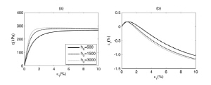
하고, 조립재료의 bounding surface 응력비에 적합하도록
 를 변화함에 따른 모델 시뮬레이션 결
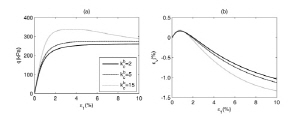
과를 Fig. 3은  와
와  공간내에서 보여주고 있다.
Fig. 3에 나타난 바와 같이  의 증가는 전단응력의 최고
치의 증가를 가중시키며, 그림에서 볼 수는 없지만 상태변수  의 전개속도를 증가시키게 된다. 이는 재료가 한계상태에 급속히 이르게 됨을 간접적으로 나타내고, Fig. 3(b)
에서 보이는 바와 같이 소성변형률이 급격히 증가되는 현
상을 야기시킨다. 또한,  의 증가는
의 증가는  공간에서 낙타
등 모양의 험프(hump)를 발생시켜 strain-softening 거동을
예측할 수 있게 한다.
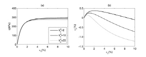
파라미터  는 dilatancy back-stress ratio
  의 값의 전개속도를 제어하며 모델내의 체적거동을 수축 또는 팽창으로 정의한다. 또한,
  는 모델의 체적변형률 거동과 비관계유동법칙의 거동을 야기시킨다. Fig. 4는 Table 2의 파
|
|
(a) | (b) |
Fig. 3. Effect of | |
|
|
(a) | (b) |
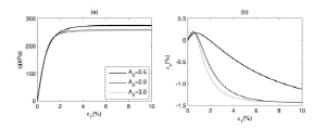
Fig. 4. Effect of | |

 on predicted drained compression response : (a)
  and (b)

 on predicted drained compression response : (a)
  and (b)
라미터를 기본으로 사용하고  의 변화
의 변화
에 따른  와
와  공간내에서 모델의 거동경향을
보여준다.  는 체적변화에 영향을 미치는 모델정수로서 체적팽창의 속도를 정의하며 둥근 조립질 재료에서는 약 10~25정도의 값이 타당하다. 모델내에서
  값의 변화가 Fig. 4(a)의
  거동에는 큰 영향을 미치지 않으나, Fig. 4(b)로부터 체적팽창거동에 상당한 인자로 작용함을 알 수 있다. 즉,
  값의 증가는 적은 전단변형률 수준에서 체적팽창을 발생하도록 모델을 제어하게 된다.
4.2 항복곡면 파라미터  , 등방경화 파라미터
  , 이동경화 파라미터
파라미터  은 순수 탄성영역을 응력비로 정의한다. Fig. 2는 항복곡면의 개요도를 보여주며, 파라미터
  은
은  값의 전개함수를 정의하며 모델 내에서 등방경화를 발생하게 한다. 일반적으로 토사재료는 순수탄성영역이 매우 작으므로 본 연구에서는
  로 가정하였고,
  로 설정하여 등방경화가 발생되지 않는 것으로 가정하였다.
파라미터  는 응력비 경로내에서 응력상태를 나타내는 대비응력텐서(back-stress tensor)
  의 전개를 정의한다. 대비응력텐서
  의 전개는 모델이 bounding surface 모델군의 하나임을 나타내며,
  는 현재 응력상태와 bounding surface에 투영된 “image”상태의 거리를 파악하여 소성계수를 결정하는데 이용된다.
  값의 증가는 소성계수의 증가와 소성 변형률의 감소를 야기시키게 된다.
Fig. 5는 Table 2의 파라미터를 사용하고 
|
|
(a) | (b) |
Fig. 5. Effect of | |
|
|
(a) | (b) |
Fig. 6. Effect of | |

 on predicted drained compression response : (a)
  and (b)

 on predicted drained compression response : (a)
  and (b)
 로 변화함에 따른
  와
와  공간 내에
공간 내에
서 모델의 거동경향을 보여준다.  값은 재료실험을 통해
산정하기 어려운 모델 고유의 양의 정수로서  값
값
을 적용한다. Fig. 5(a)의  결과로부터
결과로부터  값의 증가는 응력-변형률 거동을 보다 경직(stiff)되게 하는 결과를 발생시킴을 알 수 있고, 이는 소성계수의 증가와 소성 변형
률의 감소를 야기시키게 된다. 또한, Fig. 5(b)의  결
결
과로부터  값의 증가와 체적팽창의 양이 연관됨을 알 수
있다.
4.3 Dilation 파라미터 
조립재료의 체적거동 모델링은 구성모델의 중요한 요소로서 MD모델 내에서 체적거동은 식 (5)에 나타난 비관계유동법칙의 정의와 식 (20)의 변수 D의 전개에 따라 변화하게 된다.  일 경우 식 (20)은 Rowe's stress- dilatancy 이론에 부합된다(Wood et al., 1994).
파라미터  의 영향을 파악하기 위하여 민감도분석을 수행하였으며, Fig. 6은 Table 2의 파라미터를 사용하고
  로 변화함에 따른
  와
와  공간 내에서 모델의 거동경향을 보여준다. 변수연구를 위해
  가 1일 경우를 기준으로 임의적으로 값을 변환하였다. Fig. 6으로부터
  값의 변화는
  거동에 큰 영향을 미치지 않으나
  거동에 상당히 중요한 인자로 작용함을 알 수 있다. 즉,
  값의 증가는 체적 팽창의 전개속도를 증가시키며, 비배수 상태에서는 하중재하 초기에 유효간극수압을 많이 발생시키는 역할을 한다.
4. 결 론
본 논문에서는 조립재료(자갈)의 공학적 거동특성을 모사할 수 있는 구성모델의 주요한 파라미터들의 민감도 분석연구를 수행하였다. 조립재료의 가장 주요한 거동특성은 전단하중 하에서 체적팽창이 발생하고 응력의 방향이 바뀜에 따라 발생하는 이동경화 현상이 발생한다는 점이다. 이러한 조립재료의 주요특성을 반영하고자 Manzari and Dafalias(1997) 모델을 적용하여 각 변수들을 변화시킴에 따른 구성모델의 거동특성을 분석하였다. 분석결과 조립재료의 비관계 유동법칙을 적절히 모사할 수 있는 체적팽창 거동을 모사하기 위한  파라미터의 변화에 따라 재료의 체적변화를 모사할 수 있음을 파악하였고, 응력-변형률 거동에서 곡선의 기울기, 즉 stiffness는 이동경화 파
라미터인  을 활용하여 제어할 수 있음을 파악하였다.
또한, 조립재료의 압축상태에서  는 이동경화의 전개에
중요한 인자로 모델의 소성변형률을 지배하는 결정적인
역할을 수행하는 것으로 파악되었고,  는 모델내의 체적
거동을 결정하는 중요한 인자로 전단하중 작용시 체적팽창의 양을 제어할 수 있는 파라미터로 분석되었다. 본 연구는 조립재료를 위한 구성모델의 주요 파라미터에 대한 민감도 분석에 초점을 맞추어 수행되었으며, 향후 실제 조립재료의 실내실험결과 등을 통해 각 파라미터들을 제어함에 따라 모델의 거동을 분석할 필요가 있다.
